Abstract Land surface temperature (LST) data derived from the satellite is increasingly required to supplement the limited weather stations for assessing temperature trends in Antarctica. This study analyses the LST based on data from the Moderate Resolution Imaging Spectroradiometer (MODIS) aboard NASA’s satellite length from 2000 to 2019 at a systematic 108 sub-regions. Antarctica was divided into 12 regions, each consisting of 9 sub-regions. A cubic spline model adjusted for seasonal patterns and the autoregressive process adjusted for time series correlation. Change in LST in sub-regions was estimated by fitting the simple linear model, while cycle and acceleration were estimated using cubic spline models. Multivariate regression adjusted for spatial correlation and was used to estimate the LST increase in regions. The seasonal patterns for all 108 sub-regions were found to be quite similar. Out of 108 sub-regions, only 30 had statistically significant decreasing trends. The 12 regions showed that most temperature trends decreased, although only 5 regions were statistically significant. The results for the entire Antarctic continent showed a statistically significant decrease and a 95% confidence interval ranging from -0.668 to -0.068 °C per decade.

Keywords: Land surface temperature, MODIS, Cubic spline, Autocorrelations, Spatial correlations

Funding: We are grateful Department of Mathematics and Computer Science, Faculty of Science and Technology of Prince of Songkla University, Pattani Campus, for providing facilities to carry out this study and the Graduate School, Prince of Songkla University, Thailand, for the research funding.

Citation: Dengmasa, M., Tongkumchum, P., and Ma-A-Lee, A. 2022. Modelling MODIS land surface temperature change in Antarctica from 2000 to 2019 using cubic spline model. CMUJ. Nat. Sci. 21(4): e2022051.

INTRODUCTION

A cubic spline is a potential alternative method to model the time series of land surface temperature (LST). Recent studies have reported LST change using the cubic spline model (Wongsai et al., 2017; Devi et al., 2020; Prasetya et al., 2020; Munawar et al., 2020; Wongsai et al., 2020; Munawar et al., 2021). In the studies mentioned above, warming or cooling trends were observed at various places on both local and regional scales. However, these studies focused only on Southeast Asia, where temperature changes are affected mainly by human activities and land use or land cover change. There is overwhelming evidence that human activities, notably the burning of fossil fuels, increase carbon dioxide and other greenhouse gases in the atmosphere, causing the land surface temperature to increase. The temperature is warmest for places covering urban and built-up land, whereas it is coolest for places covering water bodies and forests. Apart from human activities, climate change is also affected by natural mechanisms. In places like the Arctic and Antarctic continents, climate changes mainly occur due to natural mechanisms. The question of whether the sensitivity to climate change places that are purely affected by natural mechanisms has warmed or cooled is crucial.

Antarctica, the largest ice region globally, is one of the world regions that is the most sensitive to climate change. The Antarctic ice sheet is of particular interest due to its contribution to the sea-level rise that could impact more than 200 million people living in coastal areas worldwide (Nicholls, 2011). Moreover, previous studies have found different temperature variations over Antarctic regions (Comiso, 2000; Shuman and Stearns, 2001; Steig et al., 2009). Some regions are warming while others are cooling. Over the past two decades, many studies have consistently found warming temperatures in the Antarctic Peninsula. However, findings on temperature changes in West and East Antarctica are not consistent (Shuman and Stearns, 2001; Kejna, 2003; Steig et al., 2009; Nicolas and Bromwich, 2014). The entire Antarctica temperature does not show significant warming or cooling trends (Monaghan et al., 2008; Steig et al., 2009; Schneider et al., 2012; Nicolas and Bromwich, 2014). The temperature change further raises the need to study trend patterns in this region.

Studies have also reported that temperature variations in Antarctica vary by time. In the last two decades, the temperature has been rising in the Antarctic Peninsula but falling in most parts of East Antarctica. The variability of surface temperature trends is strongly dependent on time period analyzed. Statistically insignificant increasing trends occur in most regions during 1960-2005 (Monaghan et al., 2008). During the second half of the 20^th century, the temperature at Antarctic Peninsula showed a much stronger warming trend (Vaughan et al., 2003; Turner et al., 2005). In stark contrast, there has been no warming since the late 1990s, and much weaker trends have been observed elsewhere in Antarctica (Turner et al., 2016; Ludescher et al., 2016; Gonzalez and Fortuny, 2018). Current temperatures at West Antarctica and Antarctic Peninsula have warmed in the second half of the 20^th century. However, in the first two decades of the 21^st century, a striking reversal of the temperature trend was observed (Turner et al., 2016; Oliva et al., 2017; Clem et al., 2020). Although previous studies suggest slight continental warming, the Antarctic continent covers an area larger than Europe. Therefore, there is a naturally marked spatial variation in temperature trends. Many long-term measurements from Antarctic research showed no significant warming or cooling trends, and temperatures have been relatively stable in most of the continent over the past few decades. Attempting to develop a long-term temperature trend for the whole Antarctic continent is almost meaningless because there is no long-term in situ temperature measurements for large areas. The trends from the various stations showed a spatially complex picture of change on the continent during the last decade and did not indicate consistent warming or cooling (Walsh et al., 2002).

A limitation of the Antarctic weather station is that temperature records were mainly based on a few stations, which are mostly located in the coastal region. Surface temperature distributions also vary from station to station, and the trends may differ even at adjacent stations (Jacka and Budd, 1998). Previous air temperature analyses may have significant errors because of the limitation of available in situ observations and large seasonal and inter annual variability in regional air temperature (Rutherford et al., 2005). Recently, satellite data sets are freely available and have been of high interest to the scientific community. Satellites have provided complete spatial coverage of various parameters in a landscape. They see the entire landscape and can make precise measurements of any location. These satellite data with high temporal and spatial resolution offer several opportunities to research and monitor climate change on local and regional scales. Therefore, much attention has been paid to the use of remote sensing-based land surface temperatures.

In this study, LST products derived from the Moderate Resolution Imaging Spectroradiometer (MODIS) aboard Terra spacecraft have been used to detect temperature variations and trends in Antarctica. The main objective of this study is to analyse LST across Antarctica in recent decades (March 2000 to February 2019) using a daytime LST (MOD11A2) product. The MOD11A2 product provides an average eight-day per-pixel LST with a 1-square kilometre spatial resolution, considering only the grounded ice sheet or mainland. Statistical methods were applied to adjust seasonal patterns, time series autocorrelation, and spatial correlation across spaces. The long-term trend patterns of LST were detected using linear and cubic spline models. The analysis was performed at the sub-regional level, regional level, and the entire Antarctic continent.

MATERIAL AND METHODS

Study area

The study area is in Antarctica. It is the southernmost continent, overlying the south pole with a parallel latitude on the Earth at approximately 66.5° south of the equator, as shown in Figure 1. Ninety-eight percent of the land surface of Antarctica is covered by ice which averages at least 1.6 km in thickness. The land surface area of Antarctica is approximately 14 million km². However, in this study, only grounded ice or mainland was considered.

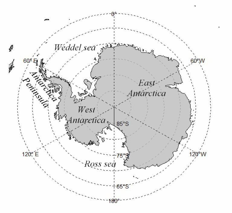
 Figure 1. Map of Antarctica continent.

Data source

The LST data have been collected by NASA’s MODIS, which flies onboard the Terra satellites (NASA LP DAAC, 2017). An eight-day daytime LST (MOD11A2) product with 1 km² spatial resolution is a tile of daily LST product gridded in the sinusoidal projection freely downloaded from the global subset tool were used. Nineteen years of data from March 2000 through February 2019 were downloaded from MODIS (https://modis.ornl.gov/cgi-bin/MODIS/global/subset.pl).

Sample survey design

The sample locations used to predict LST change in Antarctica are shown in Figure 2. According to the MODIS sinusoidal grid system, a sub-region comprising 49 pixels of dimension 7×7 pixels was selected to be included in a sample. The sub-region location was horizontally and vertically 3.357 apart according to geographic coordinate in decimal degrees. The 108 sub-regions were chosen for covering the Antarctic mainland. Some sub-regions were moved to ensure that they reside on the land. A group of nine neighbouring sub-regions were combined into a larger area and called a region. The regions are denoted with a red circle. One circle comprises nine green dots, and each dot represents one sub-region. Altogether, 12 regions cover Antarctica’s mainland, namely A, B, C, D, E, F, G, H, I, J, K and L. The LST data were retrieved individually for 108 sub-regions from March 2000 to February 2019 in eight-day intervals, or approximately 46 observations per year and maximally 874 observations over the 19 years. Due to technical problems with sensors, the observations were missing across the sub-regions over the period. Hence the actual total observation counts for each pixel were typically below the maximum. The LST time series data structure in each sub-region comprised at most 874 observations and 49 columns from 7×7 pixels.

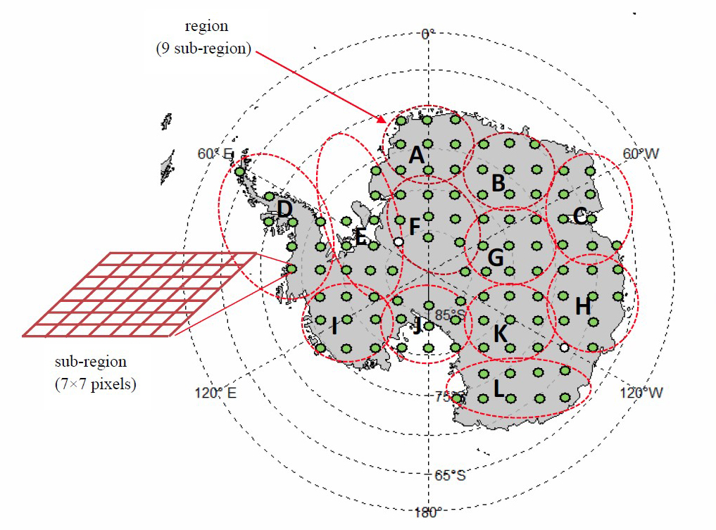
Figure 2. The study sample comprises 108 sub-regions (green point), each with a trapezoidal polygon 7 × 7 pixels. The red circle is a group of nine neighbouring sub-regions define as regions.

Statistical methods

There are inevitably missing data from MODIS due to atmospheric aerosol, clouds, or other atmospheric conditions. The LST data for each sub-region were taken as an average of 49 pixels for every observation to reduce missing values and spatial correlation and represent temperature for each sub-region. The ARIMA function in the R program (R Core Team, 2013) adjusts for time series correlation. This function uses the state-space approach (Kalman filtering) to compute the likelihood of an ARIMA model even in the presence of missing values (Durbin and Koopman, 2001; Ripley, 2002).

Cubic spline function adjusts for seasonal patterns

Like other time-series data, LST can contain some or all the four components (seasonal, trend, cyclical and irregular). The seasonal variations need to be adjusted before the analysis of the long-term trend. The cubic spline model was used to capture seasonal patterns. The spline functions are simply piecewise cubic polynomials that are linear in the distant past and future. The natural cubic spline function can extract the seasonal pattern, even when successive missing values are in the data series (Wongsai et al., 2017). Using the definition of a cubic spline (see McNeil et al., 2011; Wongsai et al., 2017), the seasonal model of LST takes the form given in (1).

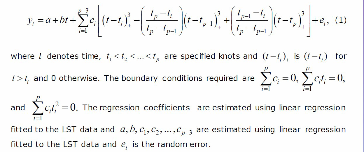
However, choosing a spacing between knots and several knots for smoothing the spline curve defines the actual cubic spline curve performance analysis. A large number of knots can result in overfitting of the data. Selecting the correct number of knots is a critical issue. Generally, more knots were placed in locations where reliable data are available. In this study, a spline with eight knots placed at day of the year 10, 40, 80, 130, 240, 290, 330, and 360, respectively, was used.

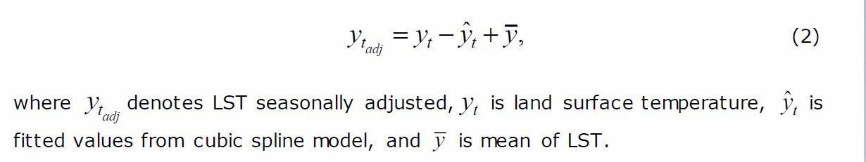
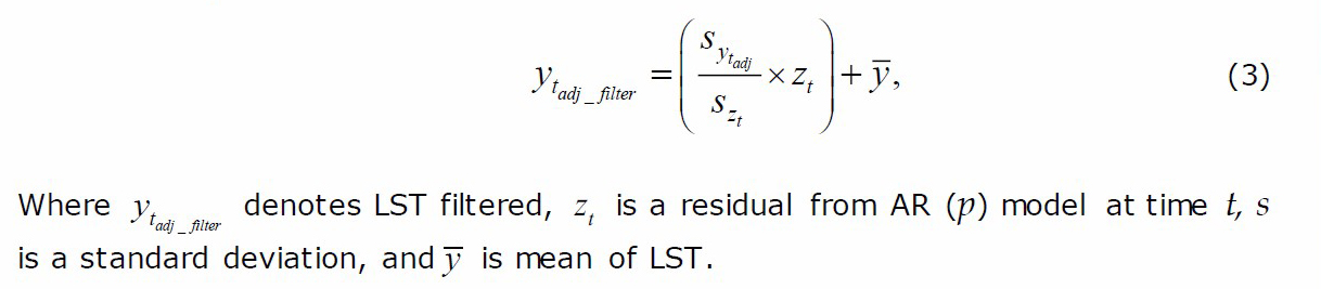
The seasonally adjusted time series of LST was computed by subtracting  the fitted values from equation (1) and adding back the mean temperature of each sub-region to obtain:

Autoregressive process

Since temperature data are time series, observations were recorded at a particular point in time. One of the assumptions in time series analysis is that the errors are independent. In particular, dependence usually occurs because of a temporal component. Error terms that are correlated over time are said to be autocorrelated. The autoregressive (AR) process was applied to account for autocorrelation among residuals of the spline model. The AR (p) is an autoregressive model of a linear combination of past values at lag 1 to lag p (see Box and Jenkins, 1970).

The LST time series were adjusted for autocorrelation using residuals from the selected AR (p) model, which is given as follows:

Linear and cubic spline models to estimate trends, cycle and acceleration

Generally, a linear regression model was used to determine the relationship between a dependent variable and one or more predictive variables. Here, LST filtered were first investigated by fitting a simple linear regression to investigate the temperature trend of each sub-region. In general, a simple linear regression has the form.

where b₀ is the intercept, b₁ corresponds to the temperature change, t  is the eight-day period, and ε_t is the error terms. The b₁ is further used to calculate the decadal LST increase.

The cubic spline model (Equation 1 without the third boundary condition) with equal spacing between seven knots at years 2000, 2003, 2006, 2009, 2012, 2015 and 2018 was fitted to the LST filtered to obtain the cyclical variations of temperature in nineteen years.

Again, the cubic spline model with equal spacing between four knots in 2000, 2006, 2012 and 2018 was fitted to the LST filtered. The four knots spline was fitted to estimate the acceleration of temperature change. The acceleration of temperature change was computed using equation (5):

where  denotes knot position with i = 1, 2, 3, 4,  and  denote the coefficient of spline four knots (Wongsai et al., 2020).

For the model validation, the adjusted r-squared and p-value from the fitted models were shown.

Multivariate linear regression

Integrating trends from sub-regions within the same region were estimated using the multivariate linear regression model. However, dynamic relationships within and between sub-regions or regions distributed across space are called spatial correlations. It has been agreed that residual spatial correlation can have a substantial impact on modelling processes and inferences. A multivariate linear regression model (Mardia et al., 1979) was used to estimate the temperature increase in the region by taking spatial correlations into account. In general, multivariate linear regression has the form.

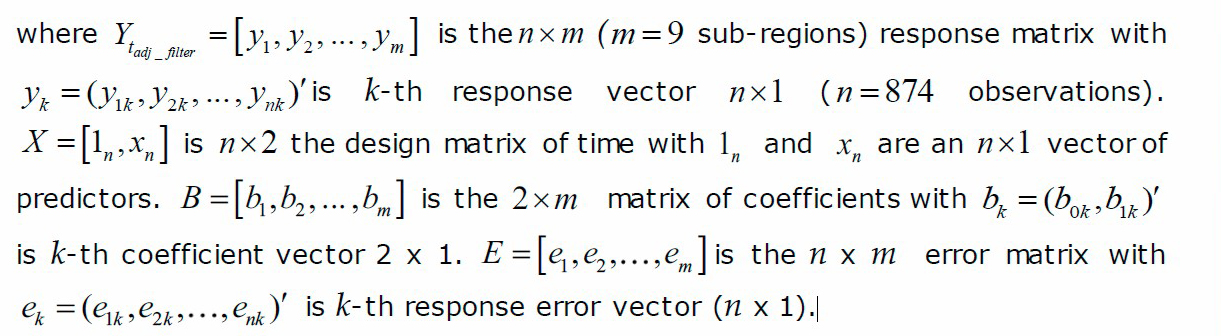
The standard error of the mean of the multivariate model was used to account for spatial correlation. The standard error (SE) takes this form in equation (7):

where Vaj_ir is the variance-covariance matrix of estimates between sub-region i  and j.  

This model (6) provides variance-covariance matrices of the estimated temperature change (increase or decrease) in the sub-region. Thus, confidence intervals (CI) for linear combinations of change were obtained. The results from the model were presented based on 95% confidence intervals and z-score.

where  Inc is the average of coefficients (B) from the equation (6) and SE is the standard error calculated from equation (7).

The LST increase in sub-region and region was estimated. A thematic map was also created using five colours to code different LST change levels for the sub-region (points) and the region (polygons) based on the z-score level. The “increase” category was divided into five levels: Increase with z > 1.96 (red), likely increase with z > 1 (orange), stable with |z| ≤ 1 (green), likely decrease with z < -1 (cyan) and decrease with z < -1.96 (blue).

All graphical displays, statistical analysis and maps are performed using the R program (R Core Team, 2013).

RESULTS

The cubic spline curve fits the LST data in an annual period. Figure 3 illustrates the yearly seasonal patterns of LST for individual sub-region in region L, which cover Victoria land of part of East Antarctica. The vertical stacks denote the average temperatures on the same day for all 19 years (some values are missing), while the horizontal is time. The red curves are fitted spline models to LST data with 8 knots denoted by blue crosses. The “r-sq” label shows the adjusted r-squared value of the cubic spline model fitted to the data. The adjusted r-squared indicates how well the proposed cubic spline function was fitted to the LST data. The graph shows that seasonal variations in region L are quite similar while sub-region 5 is slightly different as it is adjacent to the coast of the Ross sea.

In the overall continent, seasonal patterns are quite similar. A U-shaped cycle over the year with the coldest temperature occurred in the middle of the year while the warmest temperature was in December and January. This indicates that the cooling period is longer than the warming period.

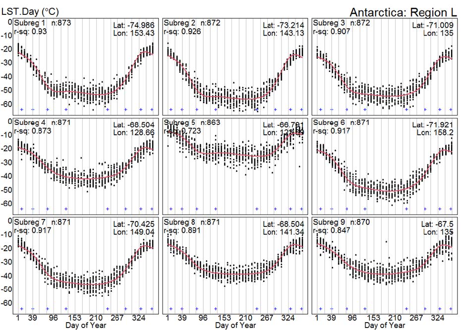
Figure 3. Example of seasonal patterns of 9 sub-regions in region L.

After obtaining the seasonal patterns for all 108 sub-regions, the seasonal effect must be adjusted before trend analysis. The random errors in the spline model of time series data are often positively correlated over time. Thus, each random error is more likely to be related to the previous random error. This autocorrelation can sometimes be detected by plotting the model residuals over time and fitting the autoregressive (AR) process. The AR process was applied to account for and filter the autocorrelation among residuals of the spline model.

The filtered temperature data for each sub-region were subjected to several models to investigate temperature trend patterns. Figure 4 illustrates the fitted models of separate nine sub-regions in region L. The grey dots represent the filtered temperature. The “ar1” and “ar2” denote the coefficients (P-value) of the AR processes at lag1 and lag2, respectively. Most of the autocorrelation considered showed that AR(2) is appropriate for AR processes. Therefore, the residual of the second-order AR process was used to adjust the LST autocorrelations. The labels “r-sq0” and “r-sq” indicate adjusted R² from the linear regression model and the seven knots cubic spline model. Larger pink dots denote outliers. The LST with a standardised residual that is larger than 9 (in absolute value) is deemed to be an outlier.

The right panel shows the comparison of linear and spline curves from the three left panels. The thin curve in the right panel showed fitted cubic splines with seven knots. The thick curve is cubic splines with four knots, while the dashed line is linear. Most of the coefficients of spline models with four and seven knots were insignificant. There is no evidence of a particular cyclic pattern within the temperature fluctuation over the past decade. The “Mean Inc/dec” indicate the rate of temperature increase (linear slope). The results from the linear model of LST in 19 years show that most of LST decreased. However, sub-regions 3, 4, 5, 8 and 9 were statistically significant. The spline coefficient with four knots was used to estimate the acceleration of temperature increase in °C per dacade², denoted as “Acc”.

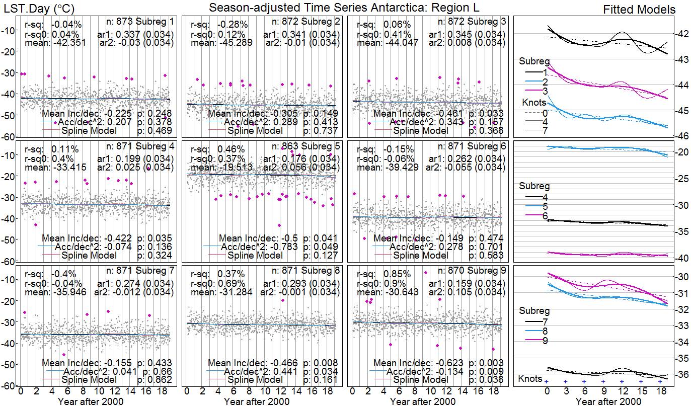
Figure 4. Example of trend patterns of 9 sub-regions in region L.

At regional level and the entire Antarctic continent, the mean day LST for the nine neighbouring sub-regions in the region was estimated using multivariate linear regression. The mean day LST for all 108 sub-regions were also estimated using multivariate linear regression to represent LST change for the entire continent. However, spatial correlation between sub-regions needs to be considered. A multivariate linear regression model was applied to combine and estimate the temperature increase in the region. The standard error of the mean from this model is taken spatial correlation into account.

To estimate LST change, the 95% confidence interval (CI) of LST change per decade for each of 12 regions and the Antarctic continent is presented in Figure 5. The 95% confidence interval, including zero, denote no significance. This is no evidence of LST change. From the result, there are 5 regions where a decrease in LST change occurred. These regions include C, D, H, I and L in range from -0.6384 to -0.0394, -0.9894 to -0.2416, -0.6989 to -0.0647, -1.0275 to -0.1690 and -0.6681 to -0.0682 °C per decade, respectively. There is no evidence of LST changes in regions A, B, E, F, G, J and K. It was also found that the entire Antarctica LST significantly decreased in the range of -0.4999 to -0.0399 °C per decade.

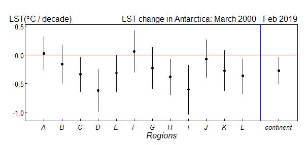
Figure 5. The 95% confidence interval of eight-day LST changes ordered by region A to L and Antarctica continent. The vertical axis shows LST change °C per decade.

Considering the entire study area, Figure 6 illustrates a thematic map of the result, using five different colours to code the different levels of LST change for the sub-region points and the regions polygons based on z-scores. At the sub-region level, the LST trends of 108 sub-regions across the study area in Antarctica are classified into five groups. The LST trend significantly decreased in 30 sub-regions (z-score <-1.96). LST will likely decrease in 17 sub-regions (z-score <-1) and likely increase in 3 sub-regions (z-score >1). LST was stable in 58 sub-regions (-1 < z-score < 1). At the regional level, the LST trends of 12 regions are also classified into five groups. The LST trend significantly decreased in regions C, D, H, I and L (z-score < -1.96), LST will likely decrease in regions E, G and K (-1.96 < z-score < -1) and LST stable in regions A, B, F and J (-1 < z-score < 1).

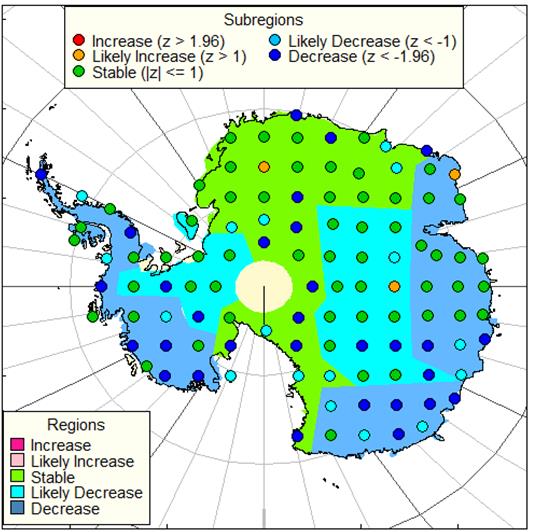
Figure 6. LST variation of each sub-region in 12 regions. The circle represents the sub-region, whereas the polygon represents the region. The circle in pink colour indicates.

DISCUSSION

In this study, the seasonal pattern of temperature Antarctic wide is quite similar. The winter season begins in March and lasts until October, while the summer season starts in October and ends in March. The seasonal patterns were quite similar in shape in the whole study as the area’s geographical features are almost indifferent. This study found that the magnitude of the temperature slightly differed depending on location. The temperature over the land of Antarctica is lower than adjacent to the coast, which agrees with the study of King (1994) and Comiso (2000), where they suggested that seasonal distribution depends on the location, altitude, and proximity to the ocean.

The analysis of temperature change in Antarctica found a significant cooling trend in the current record period from 2000 to 2019, which is consistent with the changes recorded by the Antarctic stations in recent decades. There was marked warming during the second half of the 20^th century, followed by statistically significant cooling in the first decade of the 21^st century (Turner et al., 2016; Oliva et al., 2017; Clem et al., 2018). Although the cooling trend was observed, the trend analysis is also complicated by the presence of alternating warm and cold temperatures in the region around the Antarctica continent. Several studies have shown that some areas had a warming trend while some had a cooling trend (Comiso, 2000; Doran et al., 2002; Turner et al., 2005; Chapman and Walsh, 2007).

The temperature changes in Antarctica indicate that warm and cold temperatures alternate in the sub-region around the Antarctic continent. It was also found that temperature remains stable cover in half of the sub-region sampling studied, consistent with previous studies that reported temperature trends might vary at different locations on the Antarctic continent. Some were warming, others cooling, and insignificant changes were also found (Comiso, 2000; Doran et al., 2002; Turner et al., 2005; Chapman and Walsh, 2007). The study suggests that the temperature trend in Antarctica depends on the location studied.

Moreover, this study found that temperatures decreased on the coast and west of Antarctica, while temperatures in the central and east of Antarctica remained unchanged. This is consistent with studies that reported no significant temperature change in the east of the continent. However, other studies found cooling temperature (Bracegirdle et al., 2008; Schneider et al., 2012; Nicolas and Bromwich, 2014; Turner et al., 2021). Furthermore, the temperature decreased in the west of Antarctica, which is contrary to the result from most studies that found an increase in the Antarctic Peninsula and west (Steig et al., 2009; Nicolas and Bromwich, 2014; Gonzalez and Fortuny, 2018; Turner et al., 2021). However, most of these studies used data from stations that are few and mostly located in the peripheral areas of the continent. In addition, the record of station data is longer than that of satellite data, which may affect trend analysis.

In entire Antarctica, our study found a significant cooling trend over the current record period from 2000 to 2019, consistent with changes recorded by the Antarctic stations. In recent decades, there was marked warming in the second half of the 20^th century, followed by statistically significant cooling in the first decade of the 21^st century (Turner et al., 2016; Oliva et al., 2017; Clem et al., 2018). Although a cooling trend was observed, the trend analysis was also complicated by the presence of alternating warm and cold temperatures in the region around the Antarctic continent. Previous studies of the long-term trend on the Antarctic continent indicate that there is no significant temperature change, although some studies have found cooling (Comiso, 2000; Doran et al., 2002; Turner et al., 2005; Monaghan et al., 2008; Screen and Simmonds, 2012; Nicolas and Bromwich, 2014).

The study period is also an important issue in temperature analysis of the Antarctic continent. Trend analyses show considerable sensitivity in the start and end dates (Chapman and Walsh, 2007; Monaghan et al., 2008). The Antarctica temperature trends may depend on the season and time of data observations.

The variability of the surface temperature over the Antarctic continent is related to the variability of the Southern Annular Mode (SAM) and tropical forcing (Hall and Visbeck, 2002; Thompson and Solomon, 2002; Turner, 2004; Ding et al., 2011; Ding and Steig, 2013; Clem et al., 2018). The positive polarity of the SAM is generally linked to reduced temperature variability across most of the continent.

CONCLUSION

The temperature analysis in this study based on the daytime MODIS terra daily LST product provided helpful insights into temperature variations in the Antarctic region during the first two decades of the 21^st century.

A similar seasonal pattern was observed among sub-regions. The coldest temperature occurred in the middle of the year and the warmest temperature in December and January, suggesting that the cooling period lasted much longer than the warming period. The cubic spline function has a high potential for extracting the seasonal pattern in time series data and the seasonal effects can be adjusted by subtracting its fitted values. Moreover, the AR process adjusts for time series correlation.

The trend analyses of the temperature using simple linear and cubic spline indicate variation results. The temperature is stable in the sub-regions coving about half of the sampling points, indicating that the temperature remains unchanged throughout half of the area in the Antarctic continent, mainly located in East Antarctica. The significantly changing areas in the thirty sub-regions were located in Antarctic Peninsula, and the East demonstrated a decreasing trend. According to the results of the regions, the estimation of long-term variations trend of temperature remained stable in four regions while a decreasing trend was observed in five regions. Also, the temperature of the Antarctic continent as a whole has a decreasing trend.

The timing and magnitude of the temperature variability in our results may add knowledge about climate change. It is hoped that these composite records will be beneficial to further studies in Antarctica. The proposed method is beneficial for the study of climate change in other areas.

ACKNOWLEDGMENTS

This work was partially supported by a grant from Graduate School, Prince of Songkla University. We acknowledge Emeritus Professor Don McNeil for his immense guidance during the study.

AUTHOR CONTRIBUTIONS

Maleeke Dengmasa designed the study, carried out data analysis, and carried out the manuscript writing. Phattrawan Tongkumchum assisted in performing the statistical analysis, data visualisation and manuscript writing. Arinda Ma-A-Lee assisted in checking data visualisation and manuscript writing. All authors have read and approved the final manuscript draft. Final thanks to the Language Center, Prince of Songkla University, Pattani Campus for proofreading this manuscript.

CONFLICT OF INTEREST

The authors declare that they hold no competing interests.

REFERENCES

Box, G.E.P. and Jenkins, G. 1970. Time Series Analysis, Forecasting and Control, San Francisco, CA: HoldenDay.

Bracegirdle, T. J., Connolley, W. M., and Turner, J. 2008. Antarctic climate change over the twenty first century. Journal of Geophysical Research: Atmospheres, 113(D03103): 1-13.

Chapman, W.L. and Walsh, J.E. 2007. A synthesis of Antarctic temperatures. Journal of Climate. 20: 4096-4117.

Clem, K.R., Fogt, R.L., Turner, J., Lintner, B.R., Marshall, G.J., Miller, J.R., and Renwick, J.A. 2020. Record warming at the South Pole during the past three decades. Nature Climate Change. 10: 762-770.

Clem, K.R., Renwick, J.A., and McGregor, J. 2018. Autumn cooling of Western East Antarctica linked to the tropical Pacific. Journal of Geophysical Research: Atmospheres. 123: 89-107.

Comiso, J.C. 2000. Variability and trends in Antarctic surface temperatures from in situ and satellite infrared measurements. Journal of Climate. 13: 1674-1696.

Devi, R.M., Prasetya, T.A.E., and Indriani, D. 2020. Spatial and temporal analysis of land surface temperature change on New Britain Island. International Journal of Remote Sensing and Earth Sciences. 17: 45-56.

Ding, Q., Steig, E.J., Battisti, D.S., and Küttel, M. 2011. Winter warming in west Antarctica caused by central tropical Pacific warming. Nature Geoscience. 4: 398-403.

Ding, Q. and Steig, E.J. 2013. Temperature change on the Antarctic Peninsula linked to the tropical Pacific. Journal of Climate. 26: 7570-7585.

Doran, P.T., Priscu, J.C., Lyons, W.B., Walsh, J.E., Fountain, A.G., McKnight, D.M. et al., 2002. Antarctic climate cooling and terrestrial ecosystem response. Nature. 415: 517-520.

Durbin, J. and Koopman, S. J. 2001. Time Series Analysis by State Space Methods. Oxford University Press.

Gonzalez, S. and Fortuny, D. 2018. How robust are the temperature trends on the Antarctic Peninsula. Antarctic Science. 30: 322-328.

Hall, A. and Visbeck, M. 2002. Synchronous variability in the southern hemisphere atmosphere, sea ice, and ocean resulting from the annular mode. Journal of Climate. 15: 3043-3057.

Jacka, T.H. and Budd, W.F. 1998. Detection of temperature and sea ice extent changes in the Antarctic and Southern Ocean. Annals of Glaciology. 27: 553-559.

King, J.C. 1994. Recent climate variability in the vicinity of the Antarctic Peninsula. International Journal of Climatology. 14: 357-369.

Kejna, M. 2003. Trends of air temperature of the Antarctic during the period 1958-2000. Polish Polar Research. 22: 99-126.

Ludescher, J., Bunde, A., Franzke, C.L., and Schellnhuber, H.J. 2016. Long-term persistence enhances uncertainty about anthropogenic warming of Antarctica. Climate Dynamics. 46: 263-271.

Mardia, K.V., Kent, J.T.B., and J.M. 1979. Multivariate Analysis. London: Academic Press.

McNeil, N., Odton, P., and Ueranantasun, A. 2011. Spline interpolation of demographic data revisited. Sonklanakarin Journal of Science and Technology. 33: 117-120.

Monaghan, A.J., Bromwich, D.H., and Comiso, J.C. 2008. Recent variability and trends of Antarctic near-surface temperature. Journal of Geophysical Research Atmospheres. 113(D4): 1-21.

Munawar, M., Prasetya, T.A.E., McNeil, R., and Jani, R. 2020. Pattern and trend of land surface temperature change on New Guinea Island. Pertanika Journal of Science and Technology. 28: 1517-1529.

Munawar, M., Prasetya, T.A.E., McNeil, R. and Jani, R. 2021. Sumatra land surface temperature increase. In 1st International Conference on Mathematics and Mathematics Education (ICMMEd 2020) (pp. 89-92). Atlantis Press.

NASA LP DAAC, 2017. MODIS Net Primary Productivity (MOD11A2) Version 6. NASA EOSDIS Land Processes DAAC, USGS Earth Resources Observation and Science (EROS) Center, Sioux Falls, South Dakota. (https://lpdaac.usgs.gov/dataset_ discovery/modis/modis_products_table/mod11a2). (Accessed 20 January 2019).

Nicolas, J.P. and Bromwich, D.B. 2014. New reconstruction of Antarctic near-surface temperatures: multidecadal trends and reliability of global reanalysis. Journal of Climate. 27: 8070-8093.

Nicholls, R.J. 2011. Planning for the impacts of sea level rise. Oceanography. 24: 144-157.

Oliva, M., Navarro, F., Hrbáček, F., Hernandéz, A., Nývlt, D., Pereira, P., Ruiz-Fernández, J., and Trigo, R. 2017. Recent regional climate cooling on the Antarctic Peninsula and associated impacts on the cryosphere. Science of the Total Environment. 580: 210-223.

Prasetya, T.A.E., Agung, T., Chesoh, S., Lim, A., and McNeil, D. 2020. Systematic measurement of temperature change in Sumatra Island: 2000-2019 MODIS data study. Journal of Climate Change. 6: 1-6.

R Development Core Team. 2013. R: A language and environment for statistical computing. Vienna: R Foundation for Statistical Computing.

Ripley, B.D. 2002. Time Series in R 1.5.0. R news. 2: 2-7. 

Rutherford, S., Mann, M.E., Osborn, T.J., Briffa, K.R., Jones, P.D., Bradley, R.S., and Hughes, M.K. 2005. Proxy-based northern hemisphere surface temperature reconstructions: sensitivity to methodology, predictor network, target season and target domain. Journal of Climate. 18: 2308-2329.

Schneider, D.P., Deser, C., and Okumura, Y. 2012. An assessment and interpretation of the observed warming. Climate Dynamics. 38: 323-347.

Screen, J.A. and Simmonds, I. 2012. Half‐century air temperature change above Antarctica: observed trends and spatial reconstructions. Journal of Geophysical Research: Atmospheres. 117(D16): 16108.

Shuman, C.A. and Sterns, C.R. 2001. Decadal-length composite inland west Antarctic temperature records. Journal of Climate. 14: 1977-1988.

Steig, E.J., Schneider, D.P., Rutherford, S.D., Mann, M.E., Comiso, J.C., and Shindell, D.T. 2009. Warming of the Antarctic ice-sheet surface since the 1957 international geophysical year. Nature. 457: 459-462.

Thompson, D.W. and Solomon, S. 2002. Interpretation of recent southern hemisphere climate change. Science. 296: 895-899.

Turner, J., Lu, H., White, I., King, J.C., Phillips, T., Hosking, J.S., Bracegirdle, T.J, Marshall, G.J, Mulvaney, R., and Deb, P. 2016. Absence of 21^st century warming on Antarctic Peninsula consistent with natural variability. Nature. 535: 411-415.

Turner, J., Colwell, S.R., Marshall, G.J., Lachlan‐Cope T.A, Carleton, A.M., Jones, P.D. et al., 2005. Antarctic climate change during the last 50 years. International Journal of Climatology. 25: 279-294.

Turner, J., Lu, H., King, J., Marshall, G.J., Phillips, T., Bannister, D., and Colwell, S. 2021. Extreme temperatures in the Antarctic. Journal of Climate. 34: 2653-2668.

Turner, J. 2004. The El Niño-southern oscillation and Antarctica. International Journal of Climatology: A Journal of the Royal Meteorological Society. 24: 1-31.

Vaughan, D.G., Marshall, G.J., Connolley, W.M., Parkinson, C., Mulvaney, R., Hodgson, D.A., King, J.C, Pudsey, C.J., and Turner, J. 2003. Recent rapid regional climate warming on the Antarctic Peninsula. Climatic Change. 60: 243-274.

Walsh, J.E., Doran, P.T., Priscu, J.C., Lyons, W.B., Fountain, A.G., McKnight, D.M., Parsons, A.N. et al., 2002. Recent temperature trends in the Antarctic. Nature, 418: 291-292.

Wongsai, N., Wongsai, S., and Huete, A. 2017. Annual seasonality extraction using the cubic spline function and decadal trend in temporal daytime MODIS LST data. Remote Sensing. 9: 1254.

Wongsai, N., Wongsai, S., Lim, A., McNeil, D., and Huete, A. 2020. Statistical model for land surface temperature change over mainland Southeast Asia. International Journal of Geoinformatics. 16: 33-39.

OPEN access freely available online

Chiang Mai University Journal of Natural Sciences [ISSN 16851994]

Chiang Mai University, Thailand.

https://cmuj.cmu.ac.th