Performance Evaluation Using PCA and DEA: a Case Study of the Micro and Small Manufacturing Industries in Indonesia.

 ABSTRACT Companies frequently evaluate their business performance based on existing advantages and shortcomings. Data envelopment analysis (DEA) is a useful decision-making tool for doing so; it evaluates the relative efficiency of a department or unit as a decision-making unit (DMU). It is also a powerful tool for studying production limits by using multiple inputs and outputs. Principal component analysis (PCA) is a technique for simplifying a data set by reducing multidimensional data sets to lower dimensions for analysis; it reduces the dimensions of input and output variables. This study evaluated the performance of the micro and small manufacturing industries (MSMI) in Indonesia using a combination of Principal Component Analysis and an Input-Oriented DEA Envelopment Model. Development of micro and small manufacturing industries in Indonesia is inhibited by various factors. Based on our results, we determined that the following factors were causative for MSMI in Indonesia: marketing, human resources, materials, machinery, capital and finance, product, technology, support, research & development, distribution, promotion, competitors, and policy.

Keywords: Performance evaluation, Micro and small manufacturing industries, Variable selection, PCA, DEA

INTRODUCTION

Evaluating business performance is important to a company’s growth and development. Performance evaluations aim to: (i) internally evaluate a business’ current operations and (ii) compare this performance to similar companies and best practices. This will help a company: (i) understand its strengths and weaknesses, (ii) better organize its business to meet customer demands and requirements, and (iii) define business opportunities to improve operations and activities by creating new goods, services, and processes (Cook & Zhu, 2008).

The micro and small manufacturing industries (MSMI) in Indonesia contribute to gross domestic product (GDP), create employment, and help distribute local community welfare and reduce the income gap (Putri et al., 2016a; Putri, 2016b; Putri & Abdulrahim, 2017a; Putri et al., 2017b). In 2014, Indonesia had 3.5 million MSMI, of which more than 90% were classified as micro (BPS, 2014). Several factors hinder MSMI business development: poor marketing and promotion, producing goods mismatched to market requirements, poor quality of raw materials, inadequately trained or educated employees, inappropriate fabrication facilities, manufacturing technology that does not meet modern requirements, inadequate access to capital, dependence on family and relatives, costly production, minimal innovation, inadequate distribution networks (Putri & Abdulrahim, 2017a).

This study evaluated MSMI performance in Indonesia using two methods: principal component analysis (PCA) (Zhu, 1998; Adler & Yazhemsky, 2010; Yoshino & Hesary, 2014) and data envelopment analysis (DEA) (Cook & Zhu, 2008) to help identify the problems the sector faces in developing their businesses and to identify factors to help them better compete, particularly in the face of global competition, and sustain their business.

METHODOLOGY

Theoretical background

Data envelopment analysis (DEA). Data envelopment analysis (DEA) is useful for evaluating the relative performance efficiency of departments or units as decision-making units (DMU) and to determine production limits using multiple inputs and outputs – all while reducing the need for subjective factors. Compared to other methods, its biggest advantages are that it is (i) technical, (ii) does not require a known production function with parameters in advance, (iii) is an excellent model for comparing the efficiency of different distribution networks (Yuzhi & Zhangna, 2012), and (iv) is simple to calculate and program.

Typically, businesses try to minimize inputs, such as costs, manpower, and materials; and maximize outputs, such as products, revenue, and profit. The input and output variables are selected before applying DEA. DEA uses decision making units (DMUs) to represent any business operation, process, or entity that converts multiple inputs into multiple outputs. The Data Envelopment Analysis model, created by Charnes, Cooper, and Rhodes (Charnes et al., 1978), provides a way to identify this piecewise linear frontier. Mathematical programming tools are used to identify non-dominated DMUs and create piecewise linear sections that make up the frontier. The DEA frontier is identified and fulfilled after identifying the efficient DMU; i.e., the efficient frontier consists of a DMU that performs well. By comparing each DMU with the identified efficient frontier, the DEA provides: (i) an efficiency rating (score) for each DMU, (ii) an Efficiency Reference Set (ERS), or peer group, for each unit that is not efficient; and (iii) targets for each DMU to achieve efficiency. The DEA provides information on how the inputs could be optimized and outputs im- proved if the DMU were efficient – in essence, guidelines to improve productivity and performance by using the efficient frontier.

Selection of input and output variables for DEA. With the DEA model, it is important to carefully select the input and output variables (Paradi et al., 2004). Principal component analysis (PCA) helps reduce the dimensions of these variables. PCA is a standard data reduction technique that extracts data, removes redundant information, highlights hidden features, and visualizes the main relationships that exist between observations. It is a technique for simplifying a data set by reducing multidimensional data sets to fewer dimensions for analysis (Yoshino & Hesary, 2014). Zhu (1998) was the first to use PCA to evaluate the efficiency of a DEA model by combining variables from multiple inputs and outputs. Adler and Yazhemsky (2010) reduced the dimensionality of the variables by combining PCA and DEA.

Input-oriented DEA envelopment model. There are different ways to displace the inefficient DMUs onto the frontier. This can be approached from two basic directions – those oriented to inputs or outputs. One tries to reduce inputs relative to fixing outputs at current levels. The other tries to increase outputs relative to fixing inputs at current levels (see Fig. 1). The following DEA model (1) is oriented to inputs, which are minimized while outputs are fixed at current levels:

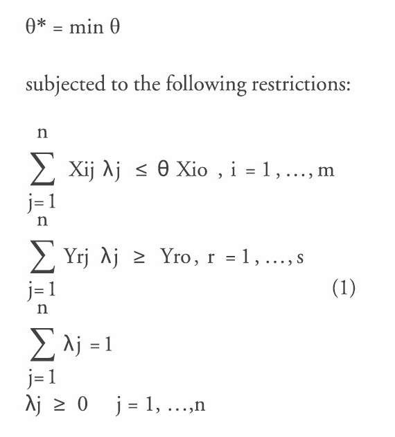
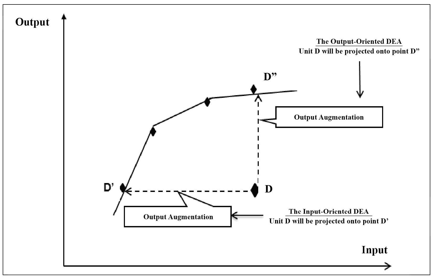
Figure 1. Formation and change of DEA frontier by input and output variables.

where DMU₀ is one of the n defined DMUs; Xi0 and Yr0 are the i^th input and the r^th output for DMU0, respectively; and λj present unknown weights, where j = 1,…, n determines the DMU number. Here, θ is a solution variable, representing the DEA effectiveness score. Because θ = 1, it is a feasible solution for model (1), with the optimal value, θ*≤ 1. If θ* = 1, then the current input levels cannot be decreased proportionally; this shows the location of DMU₀ on the frontier. If θ* < 1, then DMU₀ is found by the frontier and inputs can be decreased by the same proportion of θ*; thus, the same output levels can be achieved with fewer inputs (Cook & Zhu, 2008).

Principal component analysis (PCA). In various applications of DEA, the number of input and output variables exceeds the number of decision-making units (DMU). This is an important pitfall. Although increasing the number of DMUs can overcome this problem, this is impractical if the available DMUs are limited. In these cases, it is more reasonable to reduce the number of input and output variables (Cooper et al., 2007; Tolooa & Babaeeb, 2015). PCA helps simplify the data by removing the data from multidimensional data sets by: (i) removing data with excessive information, (ii) displaying data with hidden features, and (iii) visualizing relationships between the observed data (Yoshino & Hesary, 2014).

Cause and effect diagram. A cause and effect diagram (Ishikawa diagram) can classify the processes and parameters to be studied (Ishikawa, 1985; Simanovaa & Gejdosb, 2015). Key causal analysis can be applied to study the causes of a given event. The relative causes for a special task are divided into categories and presented in diagrams (Ishikawa, 1991; Dobrusskin, 2016). The main problems of business activities are classified into six classic categories: people, management, processes, environment, materials, and equipment (Ishikawa, 1986; Bose, 2012).

Data sample for case study

Definition of micro and small manufacturing industries. According to the Republic of Indonesia law number 20, 2008, micro and small manufacturing businesses are defined as follows (UURI, 2008):

• Micro manufacturing industries are productive business owned by an individual and/or individual business entity that has a net worth of IDR 50 million (excluding land and buildings) or annual sales of at most IDR 300 million.
• Small manufacturing industries are stand-alone productive economic enterprises owned by an individual or business entity that is neither a subsidiary nor branch, directly or indirectly, of a medium or large company that has a net worth of IDR 50-500 (excluding land and buildings) or annual sales of IDR 300 million–2.5 billion.

Industry classification according to KBLI. This study used the Klasifikasi Baku Lapangan Usaha Indonesia (KBLI) rev. 4 Tahun 2009 classifi- cation of industries (BPS, 2014), as shown in Table 1. The industries were equated to DMUs for DEA analysis.

Input and output variables. We selected four types of input data – (i) number of establishments, (ii) number of workers, (iii) input cost, and (iv) labor cost – and two types of output data – (i) value of gross output and (ii) value added (at market price) – over a six-year period (2010-15), for a total 24 input variables and 12 output variables. The input and output variables are shown in Table 2.

The actual input and output data used for analyzing the micro and small manufacturing industries are shown in Tables 3-6.

Table 1. Classification of industries according to KBLI.

Source: BPS, 2014.

Table 2. Input and output variables for the micro and small manufacturing industries 2010-15.

Source: BPS, 2014.

Table 3. Actual input data for micro manufacturing industry 2010-15.

Source: BPS, 2014.

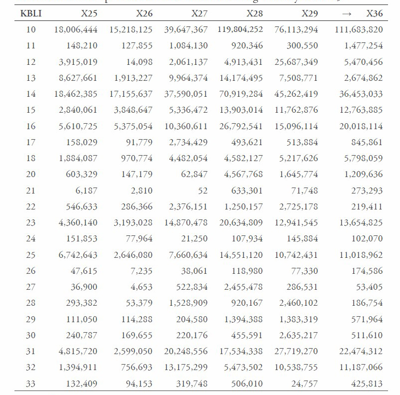
Table 4. Actual output data for micro manufacturing industry 2010-15.

Source: BPS, 2014.

Table 5. Actual input data for small manufacturing industry 2010-15.

Source: BPS, 2014.

Table 6. Actual output data for small manufacturing industry 2010-15.

Source: BPS, 2014.

Analysis

This study evaluated the performance of the micro and small manufacturing industries (MSMI) in Indonesia using a combination of factor analysis to select the input and output variables and performance evaluation.

Factor analysis for input and out-put variable selection. This study used SPSS to conduct the principal component analysis (PCA). Factor analysis was applied to reduce the data to eliminate highly correlated variables.

The principal component  method of extraction started by determining the linear combination of variables or components that counted for the greatest variation in the original variables. Next, PCA determined the other components that accounted for the greatest remaining variation that were uncorrelated with the previous components. This continued until the number of components equaled the number of original variables.

Performance evaluation uses DEA method. An input-oriented DEA envelopment model was used to obtain an optimal solution using Microsoft Excel and Solver software. Based on the optimal solution for the efficiency score, the causative factors of efficient and inefficient DMU-KBLI were then determined by applying a cause and effect diagram to analyze marketing, human resources, materials, machinery, capital and finance, product, technology, support, research & development, distribution, promotion, competitors, and policy variables.

RESULTS

Factor analysis for input and output variable selection

Input variable selection. The communalities of each variable exceeded 78%. Total variance-explained had initial eigenvalues greater than 1 for the extracted components 1 and 2. Based on the initial eigenvalues for the variance-explained, the value of summary percentage variance for the micro manufacturing industry (MMI) was equal to 97% and the small manufacturing industry (SMI) was equal to 95%. The values indicated that these two extracted components explained nearly 97% and 95% of the variability in the original 24 input variables for MMI and SMI, respectively. There- fore, we can considerably reduce the complexity of the data set by using these components, with only 3% loss of information for MMI and 5% loss of information for SMI. Table 7 de- scribes the results of total variance-explained.

The component matrix extracted two components, namely, components 1 and 2. It showed the correlations between the independent variables and these two extracted components. The correlation value between the variables and selected components was greater than 0.1. This indicated that the input selected variables for MMI were X6, X12, X16, and X20; and for SMI were X3, X9, X18, and X21.

Table 7. Total variance-explained.

Source: BPS, 2014.

Output variable selection. The communalities of each variable exceeded 87%. Total variance explained had initial eigenvalues greater than 1. The extracted component formed in this study consisted of only one component, namely, component 1. Based on the initial eigenvalues of the variance explained, the value of percentage variance for the factors explains 98% of the value of the variables in the micro manufacturing industry and 92% in the small manufacturing industry. Only one component was extracted from the rotated component matrix result, indicating that the solution could not be rotated. The correlation value between the variables and components selected in the component score coefficient matrix was greater than 0.08, indicating that the output selected variables were X30 and X36 for MMI and X28 and X34 for SMI.

Performance evaluation

Factor analysis yielded four input and two output selected variables for each industry type: (a) Micro manufacturing industry (MMI) – input1 (X6)-number of establishments, in- put2 (X12)-number of workers, input3 (X16)-input cost, input4 (X20)-labor cost, output1 (X12)-value of gross out-put, and output2 (X12)-value added; and (b) Small manufacturing indus- try (SMI) – input1 (X3)-number of establishments, input2 (X9)-number of workers, input3 (X18)-input cost, input4 (X21)-labor cost, output1 (X28)-value of gross output, and out- put2 (X34)-value added.

Table 8 shows the efficiency values of MMI and SMI (DMU-KBLI) based on the selected input and output variables. Values over 0.8 were considered efficient.

The PCA- and DEA-based estimates demonstrated that it was possible to classify the DMUs into eight categories: efficient MMI, inefficient MMI, efficient SMI, inefficient SMI, efficient MMI – efficient SMI, inefficient MMI – inefficient SMI, efficient MMI – inefficient SMI, and efficient SMI – inefficient MMI. The DMU-KBLI classification and its percentage composition for each type of manufacturing industry are shown in Table 9.

To improve the DMU-KBLI activities identified as inefficient requires reducing the input variables; the reduction amount can be found from the values of the weak input variables in Table 10.

Table 8. Efficiency and inefficiency values of MMI and SMI based on the selected input and output variables.

Table 9. DMU-KBLI classification of MSMI and its percentage composition.

Table 10. Values of the weak input variables for the micro and small manufacturing industry (MSMI).

DISCUSSION

Our study used PCA to select the input and output variables based on the same concept found in Zhu (1998), Adler and Yazhemsky (2010), and Yoshino and Hesary (2014), applying this to evaluate the performance of the micro and small manufacturing industries in Indonesia. We compared the rotated component and component score coefficient matrices to select the variables with the greatest values. In the absence of a conventional rule, a dilemma arose in selecting the variables if they had the same value.

We used a similar DEA approach as Cook and Zhu (2008) in Equation (1) to transform the inefficient DMU-KBLI activities into efficient ones. However, we differed on the calculation of weak input variables. Using their approach, we defined the values of the weak input variables X6, X12, X16, and X20 for DMU10-KBLI20, DMU11-KBLI21, DMU12-KBLI22, and DMU16-KB LI26 in micro manufacturing industry (MMI) as 0.

We had to overcome the limitations of the Cook and Zhu approach, im- proving the weak input variables and minimizing the number of input variables. The values were as follows: DMU10-KBLI 20 (X12 = 6,770; X16 = 621,752), DMU11-KBLI 21 (X6 = 873), and DMU12-KBLI 22 (X6 = 1,809; X16 = 457,974).

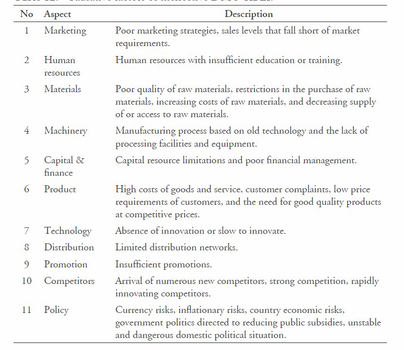
To improve the efficiency of DMU- KBLI activities, causative factors must be considered; the common factors are listed in Tables 11 and 12. Based on our results, we determined that the following factors were causative for MSMI in Indonesia: marketing, human resources, materials, machinery, capital and finance, product, technology, support, research & development, distribution, promotion, competitors, and policy. The information presented in these tables can be used as the benchmark to determine the internal factors (strengths and weaknesses) and external factors (opportunities and threats) of MSMI businesses and in order to further develop them.

Table 11. Causative factors of effective DMU-KBLI.

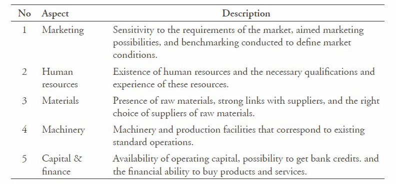
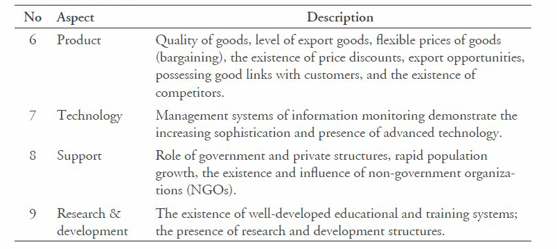
Table 12. Causative factors of ineffective DMU-KBLI.

The estimations using PCA and DEA methods in this study demonstrated that it is possible to newly classify DMU groups, and offers potential for improving DMU efficiency. The results of this study can also be used by the government as a base to formulate development strategies for MSMI in Indonesia.

ACKNOWLEDGEMENTS

This work was supported by the Research Unit on System Modeling for Industry (Grant No.SMI.KKU 572001/2558) Khon Kaen University, Thailand and the International Relations Division of Khon Kaen University, Thailand, which provided the first author with a University Scholarship for ASEAN and GMS Countries’ Personnel for academic year 2015.

REFERENCES

Adler, N., & Yazhemsky, E. (2010). Improving discrimination in data envelopment analysis: PCA–DEA or variable reduction. European Journal of Operational  Research, 202, 273–284. https://doi.org/10. 1016/j.ejor.2009.03.050

Bose, T.K. (2012). Application of fishbone analysis for evaluating supply chain and business process- A case study on the St. James Hospital. International Journal of Managing Value and Supply Chains (IJMVSC), 3(2), 17-24. https://doi.org/10.5121/ijmvsc.2012. 3202

BPS. (2014). Profile of micro and small industry in 2014 (Profil industri mikro dan kecil tahun 2014), Katalog BPS 6104006, BadanPusatStatistik, Jakarta, Indonesia.

Charnes, A., Cooper, W.W., & Rhodes,E. (1978). Measuring the efficiency of decision making units. European Journal of Operational Research, 2(6), 429–444. https://doi.org/10. 1016/0377-2217(78)90138-8

Cook, W.D., & Zhu, J. (2008). Data envelopment analysis: Modeling operational processes and measuring productivity. CreateSpace Independent Publishing Platform.

Cooper, W.W., Seiford, L.M., & Tone, K. (2007). Introduction to data envelopment analysis and its uses with DEA-solver software and references, 2^nd ed., Springer, U.S.A.

Dobrusskin, C. (2016). On the identification of contradictions using cause effect chain analysis. Procedia CIRP 39, 221–224. https://doi. org/10.1016/j.procir.2016.01.192 Ishikawa, K. (1985). What is total quality control? The Japanese way (1 ed.). Englewood Cliffs, New Jersey: Prentice-Hall.

           . (1986). Guide to quality control. Tokyo, Japan: Asian Productivity Organization.

           . (1991). Guide to quality control. Tokyo, Japan: Asian Productivity Organization. 

Paradi, J.C., Vela, S., & Yang, Z.J. (2004). Assessing bank and bank branch performance. In: Cooper W.W., Seiford L.M., Zhu J. (eds) Handbook on Data Envelopment Analysis. International Series in Operations Research & Management Science, vol. 71. Springer, Boston, MA.

Putri, E.P. (2016b). Cluster development of small and medium manufacturing industry in Surabaya City, East Java, Indonesia. In Ivan A. Parinov, Shun-Hsyung Chang, Vitaly Yu. Topolov (Eds.). Proceedings of the 2015 International Conference on Physics and Mechanics of New Materials and Their Applications, devoted to 100-th Anniversary of the Southern Federal University. (pp. 565-570). Nova Science Publishers, New York.

Putri, E.P., & Abdulrahim M. (2017a). Business development of small and medium enterprises as poverty alleviation efforts in East Java province, Indonesia. In Ivan A. Parinov, Shun-Hsyung Chang, Muaffaq A. Jani (Eds.). Proceedings of the 2016  International  Conference on Physics and Mechanics of New Materials and Their Applications. (pp. 627-633.) Nova Science Publishers, New York.

Putri, E.P., Chetchotsak, D., Jani, M.A., & Hastijanti, R. (2017b). Performance evaluation of micro and small manufacturing industry in Indonesia. Proceedings of International  Conference  on   Simulation and Modelling (SIMMOD 2017) (pp. 82-92).

Putri, E.P., Chetchotsak, D., Ruangchoenghum, P., Jani, M.A., & Hastijanti, R. (2016a). Performance evaluation of large and medium scale manufacturing industry clusters in East Java Province Indonesia. International Journal of Technology, 7, 1117-1127. https://doi.org/10.14716/ ijtech.v7i7.5229

Simanovaa, L., & Gejdosb, P. (2015). The use of statistical quality control tools to quality improving in the furniture business. Procedia Eco- nomics and Finance, 34, 276 – 283.

Tolooa, M., & Babaeeb, S. (2015). On variable reductions in data envelopment analysis with an illustrative application to a gas company. Applied  Mathematics and    Computation, 270, 527–533. https://doi.org/10.1016/j.amc.2015.06.122

UURI. (2008). The law of the Republic of Indonesia number 20 year 2008 (Undang-Undang Republik Indonesia Nomor 20 Tahun 2008 tentang Usaha Mikro, Kecil dan Menengah).

Yuzhi, S., & Zhangna. (2012). Study of the input-output overall performance evaluation of electricity distribution based on DEA method. International Conference on Future Energy, Environment, and Materials. Energy Procedia, 16, 1517 – 1525. https://doi.org/10.1016/j.egypro. 2012.01.238

Yoshino, N., & Hesary, F.T. (2014). Analytical framework on credit risks for financing SMEs in Asia. Asia-Pacific Development Journal, 21(2), 1–21.

Zhu, J. (1998). Data envelopment analysis vs. principal component analysis. European Journal of Operational Research, 111, 50–61. https://doi.org/10.1016/S0377- 2217(97)00321-4