ABSTRACT

As efficient planning and design of transportation route can reduce transportation cost of an organization, the development of an effective algorithm for solving this problem can be used as a guideline for developing the route and transportation cost. Currently, several studies focus on the study and development of the Traveling Salesman Problem (TSP), which is largely similar to transportation route. One of the algorithms that helps solve this type of problem quickly is the Self-Organizing Map (SOM), which is adapted from the Artificial Neural Networks algorithm. However, using SOM to solve TSP problem does not provide the shortest path, nor is it the optimal solution. Therefore, this study aims to develop the solution based on SOM together with Local Search algorithm to provide better quality solution. The results of this research, both in terms of processing time and quality of solution, were compared to the results of previous research. The findings indicated that the solution from the proposed algorithm improved the processing time when compared to every problem in previous research.

Keywords: Hybrid, Traveling Saleman Problem (TSP), Self-Organizing Map (SOM), Algorithm

INTRODUCTION

Logistic costs play a significant role in the cost of goods. Transportation cost is one of the costs that needs to be highly paid. Therefore, the reduction of transportation cost is important to increase the value of goods. This will benefit and lead to the development of the industry. Transportation is an important activity in logistic system of businesses since transportation cost affects the cost of producing goods or services. By considering the supply chain system of a product or service, transportation process is the process of moving one thing from one place to another, which is an essential part of logistic activity. One crucial issue contributing to unnecessary transportation cost is transportation route planned with inefficient vehicles. Consequently, the reduction of transportation cost by providing appropriate route planning is the guideline for businesses to select the most efficient way to transport goods to customers in order to provide customer satisfaction and reduce unnecessary costs.

Traveling Salesman Problem (TSP) is one of the problems that is similar to the problem of reducing transportation costs since TSP solution is to find the lowest path or the shortest distance of all trips to customers. Since TSP problem is complex at NP-Hard level, many studies have tried to develop algorithms to find optimal solution within the shortest processing time.

Self-Organizing Map (SOM) (Kohonen, 1990) is another algorithm currently used in solving TSP, one of the algorithms that are relatively effective in finding the solution of the problem (Cochrane and Beasley, 2003). However, such solution is not always the optimal solution. In order to maximize the efficiency of finding optimal solution, the researchers aimed to use SOM and Local Search algorithm (Olli and Gardreau, 2005) to solve TSP to obtain the solution that is equal or close to optimal solution most.

Traveling salesman problem

Traveling salesman problem (TSP) is a problem of finding a way to travel to a certain number of cities and return to their original position. The aim is to make the journey as short as possible, which is a tour or a circular orbit. The mathematical modeling of this problem has the requirement to route the trip through a single trip, leave the position to get to the next until all positions are reached, and then come back to the beginning. This is comparable to a vehicle that must travel to all destinations before returning to the distribution point. Types, variables, and examples of the mathematical model of the problem can be expressed as follows:

Indices

i, j are the orders of cities or customers that need to be visited; i, j = 1,2,3,...,n

Parameters

c_ij is the distance between customer i to customer j

Decision variables

x_ij is equal to  when traveling from customer i to customer j other than that it is 0.

U_i is a variable for subtour elimination.

M is a higher value so that constraints will be true.

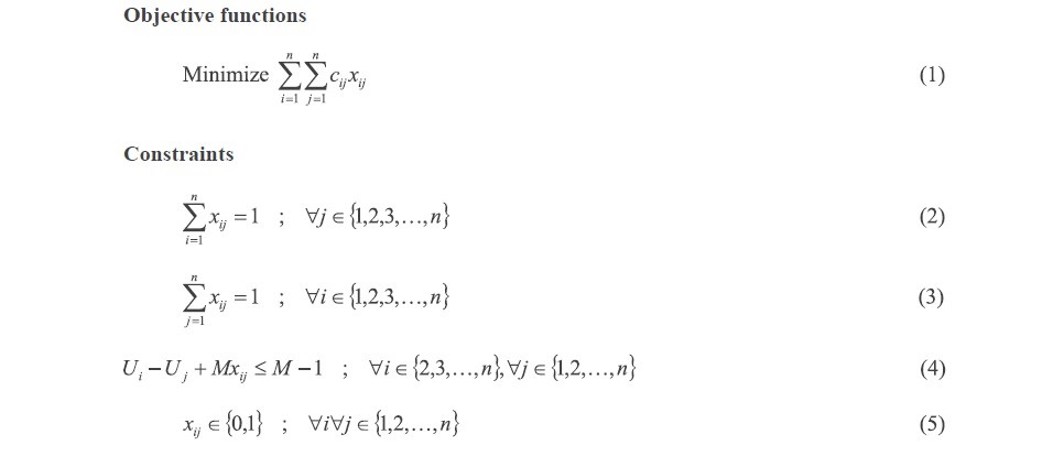
when (1) is the objective function for the shortest distance, condition (2) and (3) allow each city to be visited only once. Condition (4) will be subtour elimination, and condition (5) will determine the decision of the variables whether to select or not.

Self-Organizing Map (SOM)

Self-Organizing Map (SOM) (Kohonen, 1990), Self-Organizing Feature Map (SOFM), or Kohonen Self-Organizing Map is an algorithm developed by Teuvo Kohonen (1990), which is an artificial neural network like the human brain system. It is often used in multi- dimensional clustering or as a tool for data visualization.

The application of the artificial neural network approach in solving TSP was initiated by Hopfield and Tank (1985). The calculations are based on the lowest value obtained from the energy function and has been improved until SOM algorithm is used to solve this problem. Modares et al. (1999) proposed SOM algorithm for solving a relatively efficient TSP problem.

The learning process of SOM

The learning process of SOM is illustrated as follows:

• Select input vector randomly from input domain.
• Compare input vector xi to input vector yj of each node to find the winner node

(j) from all nodes. The winner node is the node with the most similar value with the input calculated by using the Euclidean distance function shown in Eq. (6) as follows:

• Adjust weight vector of the winner node so that it will be close to the input.
• Adjust weight vector of neighborhood nodes so that the next input vector having similar value would have a new winner node nearby as in Eq. (7) as follows:

when t is each processing round

x_i,(_t) is the input vector obtained from random input at t processing round.

α(_t) is the learning rate at t round.

F(d_j,(_t)) is the function used to determine the weight in neighborhood node adjustment. In general, Gaussian function or other functions will be employed depending on the suitability of the problem.

• Repeat step 1 through 4 until the number of cycles or conditions is reached.

In this research, SOM algorithm is applied in the above equation. The solution to that will be developed with local search algorithm.

Local search. Local search (Olli and Gendreau, 2005) is the solution to a particular problem. The map is definitely fixed, and the solution is an estimated solution, which cannot guarantee the best solution or the same solution every time. Typical local search behavior after finding initial feasible solution results generates a mechanism for changing the response, and then stops responding when acceptable values are obtained. The mechanism of changing the results for this TSP problem can be achieved by changing the position of the path that connects the two existing customers to the new route that connects the customer to the new point. If this changes results for a shorter distance than the old solution, replace the old solution with the new one. Do this repeatedly until it covers the required number of rounds or meets with acceptable conditions. In this study, the following three routes are used:

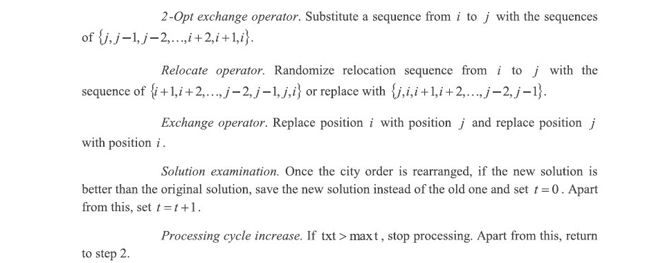
2-Opt exchange operator. 2-Opt Exchange Operator for TSP aims to reduce the distance without crossing routes. Examples of this mechanism are shown in Figure 1.

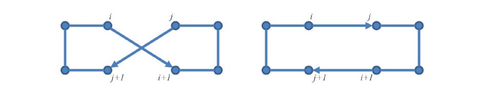
Figure 1. 2-Opt Exchange Operator mechanism will change i to i+1 and j to j+1 which is from i to j and i+1 to j+1, and other points between j to i+1 will be swapped.

Relocate operator

Relocate Operator will change two routes connected to each other at a given point without passing through it again. Then it will create a new route to that point by changing one or the other route into two routes connected to that point. Examples of this mechanism are shown in Figure 2.

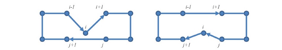
Figure 2. Relocate operator mechanism will change route i-1, i and i, i+1 to i-1, i+1 as well as route j, j+1 to j, i and i, j+1

Exchange operator.

Exchange Operator will change two routes connected to each other at a given point into two routes connected to a new point. The two old routes connected to the new point will be transformed into two routes connected to the old one. Examples of this mechanism are shown in Figure 3.

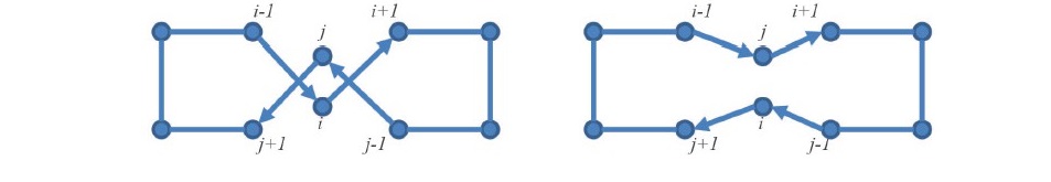
Figure 3. Relocate Operator mechanism will change route i-1, i and i, i+1 to i-1, i-1, j and j, i+1 respectively as well as route j-1, j and j, j+1 to j-1, i and i, j+1 respectively.

Self-Organizing Map algorithm and local search for problem solving

This research employs Self-Organizing Map algorithm to find out the initial solution, and uses Local Search algorithm to develop a better solution. For TSP problem with N cities, this SOM algorithm will start with creating a node to look for solutions, or neighboring M nodes, which is twice the number of cities. It is circular in shape with a circle centered randomly at the top and bottom value of each city. The variables in the algorithm are defined as follows:

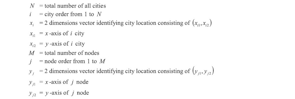
After creating a node for search, the next step is to find the winner node. This process starts with one random city in the processing cycle. Find the winning node or node closest to the nearest random city from each of the processing cycles. Finding the winning node can be calculated from the following Eq. (8)-(9).

From Eq. (8), (9), it is possible to find the winning j node from the lowest j node, ArgMinj. Then the next step is to move the position of these nodes to form a route connected between cities in the processing cycle. The position of each node is calculated by the equation as follows:

The changing position of each node in each processing cycle will make each node move to a random location in the processing cycle. The node that moves at the maximum distance is the winner node. Other nodes near the winner node will move in a decreasing distance depending on the closeness to the winner node. The d_j in Eq. 13 and function d_j in Eq. 12 and G in Eq. 12 are set to decrease with each processing round. The coefficients for determining the size of the motion of each node are given by the value of μ in equation 11.

It then sets the distance that is close enough for every city to end the algorithm. When processing it continuously, each node will move to a random city until it is similar to the route that tells traveling order of the cities. The processing stops when each city is away from any node that is less than the given distance. The result is the city order based on the closeness of the node. The proposed algorithm can be outlined as the following procedure:

Initialization. N = number of cities, M = number of nodes. Create a circular node network with randomly generated center. Set the default values of μ, G, and α as appropriate. In this research, the values are 0.1, 20, 0.99 respectively for small problems and 0.1, 100, 0.9 respectively for large problems. Create a close-enough distance for every city. Create t variable as the sequence of the processing cycles and set t = 1. Create an inhibit variable by setting Inhibit_j = 0 on each node.

City sequence random. Create a set of random city sequence.

Choose a city to process. Select the city in the t-order of the generated set.

Select the winner node. Calculate the location of the random city (x_i) to find winner node J using Eq. 8, set Inhibitj = 1 for the winner node. If t ≤ N, select the winner node from any node that Inhibit_j = 0 only.

Modification. Move every node with equation 10.

Constraint examination. If all cities are CloseEnough_i , stop processing. Apart from this, go to step 7.

Processing cycle increase. If t < N, set t = t+1 and return to step 3. Apart from this, set, t = 1, Inhibit_j = 0 on each node, and return to step 2.

SOM algorithm in this study will help to quickly find solution to TSP. The characteristics of this algorithm during each round of processing can be displayed in two-dimensional planes as shown in Figure 4.

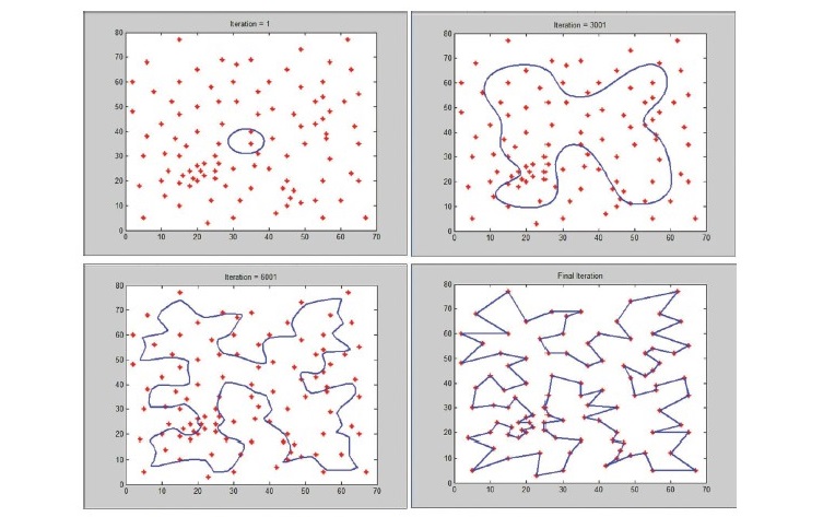
Figure 4. Examples of SOM algorithm mechanism to solve TSP.

Since the solution from SOM algorithm cannot guarantee that this is the optimal solution, chances are that the solution will be changed to the better value. As a result, the solution from SOM algorithm will be improved with Local Search algorithm. The solution given by SOM is determined as the initial solution before further improvement. In this paper, we used three local search algorithms: 2-Opt Exchange Operator, Relocate Operator, and Exchange Operator. The improvement of the initial solution can be outlined as the following procedure:

Initialization. Set t as the number of processing cycles, t = 0, set max t as the highest number of repetitions where the solution is not better, and set max t = 500,000.

Result improvement by local search. We used the sequencing results of the cities that are the best answer today, and changed the location using Randomize the improvement using one of the three Local Search methods. Each Local Search outline is assigned i and j as a random sequence of cities without redundancy, and i < j.

After developing the solution with local search, the result is usually better or shorter. The examples of the change are shown in Figure 5, where the solution will be improved from 680.1 units to 663.3 units.

Figure 5. Examples of the change in the proposed local search algorithm.

RESULTS

In this research, 20 TSPs from TSPLIB95 database were used, and small problems of no more than 1,000 cities were selected. All calculations were proceeded by using the MATLAB R2013b program, Intel^® Core™ i5-5200U CPU @ 2.2GHz RAM 8 GB. The results were compared with previous studies of Peker et al. (2013) and Zhou et al. (2015) which used different algorithms. The results were compared to the best values available, the mean of the solution, and the mean of 100 times of total processing. The comparison results with previous researches are shown in Table 1.

Table 1. Comparison of the results of proposed and previous researches.

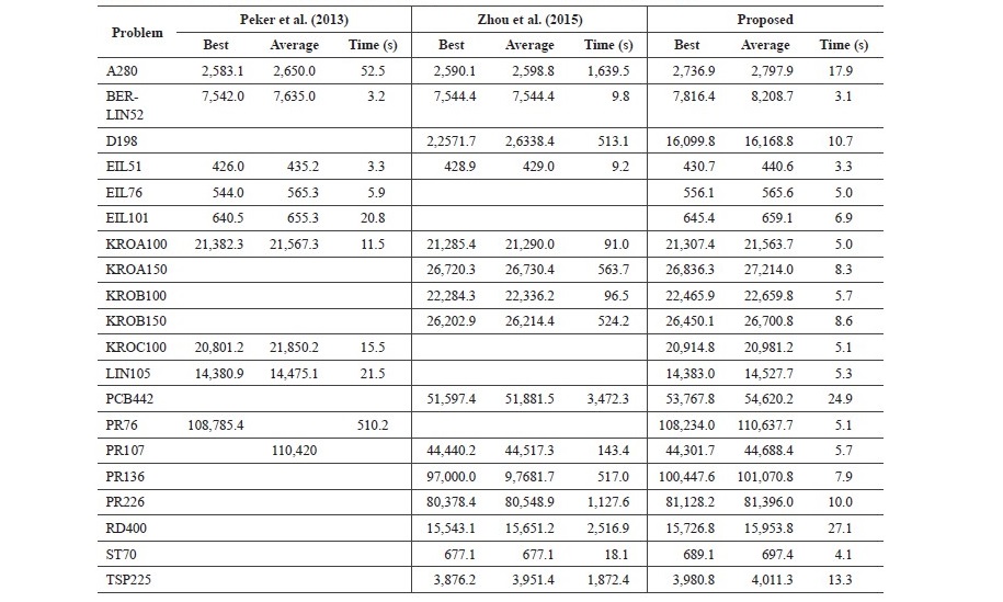
The findings showed that the quality of the solution obtained from the proposed algorithm is lower than the algorithm from the previous research. Regarding the comparison, four out of 20 problems of the proposed algorithm can find better quality solution, but when compared in terms of processing time, the proposed algorithm uses less processing time than other studies in every problem.

CONCLUSIONS

After implementing SOM algorithm with 2-Opt Operator, Relocate Operator, and Exchange Operator Local Search, the algorithm will be very efficient in terms of the processing time of solution finding since it uses less time than other algorithms in previous research, especially the problems that are large or include several cities. In comparison, the proposed algorithm is less time consuming than others. For example, for PR76 in Peker et al. (2013), it took 510.2 seconds to process, but the proposed algorithm used only 5.1 seconds. Moreover, for PCB442 in Yongquan Zhou et al. (2015), it took 3,472.3 seconds in processing time while the proposed algorithm used only 24.9 seconds.

The results of using less processing time of the proposed algorithm would be useful to apply to other algorithms, such as finding a default solution in order to further develop other algorithms. This is because the default solution obtained has a relatively good quality but is less time consuming. This helps develop an optimal solution using other algorithms with better performance.

However, the solution quality obtained from the proposed algorithm is not better than those of other studies. As a result, the following suggestions should help develop the solution with better quality.

• The positioning of the initial node may be used in a different shape other than a circular shape.

• Parameters in the algorithm, such as μ, G, and α, may not have an optimal value for each problem.

ACKNOWLEDGEMENTS

Chiang Mai University (CMU), through the research administration office, provided the funding to Excellence Center in Logistics and Supply Chain Management (E-LSCM).

REFERENCES

Cochrane, E.M., and Beasley, J.E. 2003. The co-adaptive neural network approach to the Euclidean Travelling Salesman Problem. Neural Networks. 16(10): 1499-1525. https:// doi.org/10.1016/S0893-6080(03)00056-X

Hopfield, J., and Tank, D.W. 1985. Neural computation of decisions in optimization problems.

Biological Cybernetics. 52(3): 41-52. https://doi.org/10.1007/BF00339943

Kohonen, T., 1990. The self-organizing map. Proceedings of the IEEE. 78(9): 1464-1480. https://doi.org/10.1109/5.58325

Modares, A., Somhom, S., and Enkawa, T. 1999. A self-organizing neural network approach for multiple traveling salesman and vehicle routing problems. International Transactions in Operational Research. 6: 591-606. https://doi.org/10.1016/S0969-6016(99)00015-5

Olli, B., and Gendreau, M. 2005. Vehicle routing problem with time windows, part I: Route construction and local search algorithms. Transportation Science. 39(1): 104-118. https://doi.org/10.1287/trsc.1030.0056

Peker, M., Sen, B., and Kumru, P.Y. 2013. An efficient solving of the traveling salesman problem: the ant colony system having parameters optimized by the Taguchi method, Turkish. Journal of Electrical Engineer & Computer Sciences. 21: 2015-2036. https:// doi.org/10.3906/elk-1109-44

Zhou, Y., Luo, Q., Chen, H., He, A., and Wu, J. 2015. A discrete invasive weed optimization algorithm for solving traveling salesman problem. Neurocomputing. 151: 1227-1236. https://doi.org/10.1016/j.neucom.2014.01.078