ABSTRACT One major question that arises when we talk about the elements in bones is whether all bones contain the same elements. This study was implemented to answer this question and determine what the elemental levels are in the femur bones of pigs using the handheld X-ray fluorescence technique. Ten dry femur bones taken from adult domestic pigs (Sus scrofa domesticus) were scanned using a handheld XRF analyzer. We compared three different groups in this study. First, comparisons were made between six locations of the whole femur bones as follows; compact bone at diaphysis (CD), compact bone at epiphysis (CE), spongy bone at diaphysis (SD), spongy bone at femoral head (SFH), spongy bone at femoral trochlea (SFT) and spongy bone at metaphysis (SM). Second, the different parts of the compact bones at the diaphysis were compared (proximal, middle and distal), Third, comparisons were made among four directions at the diaphysis (cranial, caudal, lateral and median). Differences in the elemental percentages and Ca/P ratio among all locations were determined by one-way ANOVA. The presence of most of the detected elements (19 from 25) in all specimens, and that the Ca/P ratio differed significantly (P<0.05) when all six parts were compared. The highest percentage in all elements was observed in CD. Notably, this data is important in terms of the elements studied. We have proven that the elements were not equally distributed throughout the bones; however, there may not be any clear effects on species classification using the elemental composition in bones.

Keywords: Distribution, Long bone, Element, XRF

INTRODUCTION 

          Species identification is an important issue in forensic science. Species identification can be effectively achieved when complete organ samples or bone samples are used (Schotsmans et al., 2017). On the contrary, incomplete specimens of the remains of bones contribute to some of the difficulties that are associated with species identification. Currently, there are many approaches used for species identification that can deliver a high degree of accuracy. Species identification can be successfully established through the use of many of these approaches using incomplete bone samples. More specifically, molecular identification (Holland and Parsons, 1999; Moore and Frazier, 2019; Pereira et al., 2019), macroscopic identification (Corrieri and Márquez-Grant, 2019), microscopic identification (Nganvongpanit et al., 2015; Cummaudo et al., 2018; Cortellini et al., 2019;  Cummaudo et al., 2019) and/or elemental composition (Nganvongpanit et al., 2016c; Nganvongpanit et al., 2017b) can all be achieved with incomplete specimens. However, each approach is associated with its own set of advantages and disadvantages. For example, the molecular technique is associated with a very high rate of accuracy. However, it requires sophisticated equipment and the expertise of knowledgeable technicians, either of which can result in increased expenses with regard to their installation and implementation. Importantly, this technique cannot be done at the scene, while the use of this method may not be appropriate in some cases or situations.

           However, the specific disadvantages mentioned above could be overcome by using a number of other techniques. These alternative methods can serve as screening tools that can be employed prior to the results being confirmed with a proper molecular technique. Our previous studies demonstrated that the use of elemental composition in dense connective tissues, such as the bones or teeth of humans and/or the bones, teeth or horns of animals, could effectively be used in species classification with a satisfactory degree of accuracy and a positive precision rate (Castro et al., 2010; Buddhachat et al., 2016a; Nganvongpanit et al., 2016a; Buddhachat et al., 2016b; Nganvongpanit et al., 2016b; Nganvongpanit et al., 2016c; Buddhachat et al., 2017; Nganvongpanit et al., 2017a; Nganvongpanit et al., 2017b). However, many other studies must be undertaken before it can be established that this method could be effectively used in the field. This is because of the limitations that are associated with this technique. Previously, it was found that different types of bones possess different elemental profiles, even in terms of major elements such as Ca and P, and the Ca/P ratio. This is indicative of the differences that can be found among different bone types (Nganvongpanit et al., 2016d). Furthermore, a previous study has addressed the limitations of the XRF technique by indicating that bones coated with lacquer could interfere with the elemental detection process when using a handheld XRF machine. Consequently, this can lead to potential alterations in the proportions of various elements on the surface of that bone (Buddhachat et al., 2019). Herein, we have attempted to prove our hypothesis that all elements might be unevenly distributed through a single piece of bone via an assessment of the elemental content. Ultimately, this assessment could then be employed as a tool for species identification.

MATERIALS AND METHODS 

Bone samples

           Dry right femur bones of ten different adult domestic pigs (Sus scrofa domesticus) were obtained from the Veterinary Anatomy and Pathology Museum, Department of Veterinary Biosciences and Public Health, Faculty of Veterinary Medicine, Chiang Mai University.

X-Ray fluorescence (XRF) measurement

          Sample elemental analyses were conducted using a handheld XRF analyzer (DELTA Premium, Olympus, USA) with a silicon drift detector that allowed researchers to detect elements from magnesium (12 Mg) through to bismuth
(83 Bi) on the periodic table. The elements below Mg were designated as light elements (LE). The collimator size was set at 0.3 mm for the analysis-area diameter, while operating voltages of 10 and 40 kV with 2 min scans were used as a source of incident radiation. X-Ray Fluorescence measurement using a handheld XRF analyzer has been used for species identification by measuring the elemental composition in bones (Buddhachat et al., 2016a; Nganvongpanit et al., 2016b; Nganvongpanit et al., 2016c), teeth (Buddhachat et al., 2016a; Buddhachat et al., 2016b; Nganvongpanit et al., 2017a; Nganvongpanit et al., 2017b) and horns (Buddhachat et al., 2016a).

Scanning location of HHXRF

           Each bone was scanned (Figure 1) at six regions including; 1-compact bone at diaphysis (CD), 2-compact bone at epiphysis (CE), 3-spongy bone at diaphysis (SD), 4-spongy bone at femoral head (SFH), 5-spongy bone at femoral trochlea (SFT) and 6-spongy bone at metaphysis (SM). All parts, with the exception of the compact bone at diaphysis, were scanned at least three times at different scanning points of each bone. The compact bone at diaphysis was scanned at 12 different points including; 1-proximal anterior, 2-proximal posterior, 3-proximal lateral, 4-proximal median, 5-middle-anterior, 6- middle posterior, 7-middle lateral, 8- middle median, 9- distal anterior, 10- distal posterior, 11- distal lateral and 12- distal middle. Each point was then scanned in triplicate.

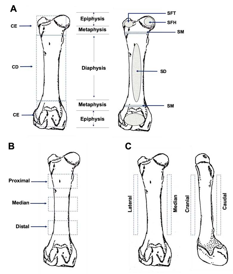
Figure 1.    Landmark of scanning on femur bone samples at 6 different locations (A), 3 different parts (B) and 4 different directions (C). CD = Compact bone at diaphysis, CE = Compact bone at epiphysis, SM = Spongy bone at metaphysis, SD = Spongy bone at diaphysis, SFT = Spongy bone at femoral trochlea, SFH = spongy bone at metaphysis 

Data and statistical analysis

          The percentages of the individual elements in each sample are presented as mean ± SD values. Moreover, Ca and P were used to calculate the Ca/P ratio. Differences in the elemental percentages and the Ca/P ratios for the different locations were assessed by one-way ANOVA with Duncan test at a P-value < 0.05. Firstly, comparisons were made among six locations of the whole femur: compact bone at diaphysis (CD), compact bone at epiphysis (CE), spongy bone at diaphysis (SD), spongy bone at femoral head (SFH), spongy bone at femoral trochlea (SFT) and spongy bone at metaphysis (SM). Secondly, comparisons were made between two different locations on the compact bone at diaphysis. This was accomplished by making comparisons between the proximal, middle and distal parts, and by making comparisons between the 4 directions including the cranial, caudal, lateral and median parts at the diaphysis. 

             Additionally, the accuracy rate of classification amongst different parts of the bone were analyzed using stepwise discriminant analysis with Wilks’ Lamda (F-level between 2.71-3.84) in order to identify the suitable elements that could be used to create an effective model. Accuracy rates were obtained from the appropriate model. In order to study the similarity of the elements in each category, heat maps (which involve a combination of dendrograms and heatmaps) were generated from the mean values of the detected elements (Engle et al., 2017; Nganvongpanit et al., 2020; Ryan  et al., 2020).

RESULTS 

Comparison of elements at different parts of femoral bones

          Our results exhibited that most of the detected elements (19 from 25), as well as the Ca/P ratio, differed significantly (P<0.05) when comparisons were made among the six parts. It was revealed that the highest percentage in all elements was observed in CD. Three elements, namely Al, Mo and W, could be found in only specific individual parts identified as CE, CD and SM, respectively (Table 1). Furthermore, the Ca/P ratio of CE was found to be significantly higher (P<0.05) than the other parts (Table 1). When comparing the elements at different locations of the diaphysis at the proximal, middle and distal, it was noted that there were only six elements of all 23 elements that exhibited a considerable difference (P<0.05) (Table 2). Mo was the single element that was detectable in only the middle part, while Mg, Ni and Zr were detected in two of the three other parts. The Ca/P ratio in the meddle part was significantly lower (P<0.05) than in the proximal and distal parts (Table 2). Across four directions of diaphysis, we found that five of the 23 elements were significantly different (P<0.05). However, the Ca/P ratio was similar in all four directions. As is depicted in Figure 2, the mean values of the percentages of all elements were presented with the use of a clustered heat map. Based on the elemental profile of six locations, the results could be separated into two groups as SM and the other remaining locations (CD SFH, CE, SD and SFT). Notably, CD revealed the highest percentage in most of the elements. When clustering was achieved using three parts, the clusters consisted of two groups; the middle and the other part (proximal and distal). Lastly, when using the elemental profiles obtained from the different directions, we noted that there were two distinct groups identified as cranial & median and caudal & lateral.

Table 1. Mean and standard derivation (SD) values of each element detected in six locations of femurs.

Note: Superscripts (a, b, c, d, e) indicate significant differences (P<0.05) between bone parts for the same element.

Table 2.   Mean and standard derivation (SD) values of each element detected in compact bones a three locations of femurs.

Note:   Superscripts (a, b, c, d, e) indicate significant differences (P<0.05) between bone parts of the same element.

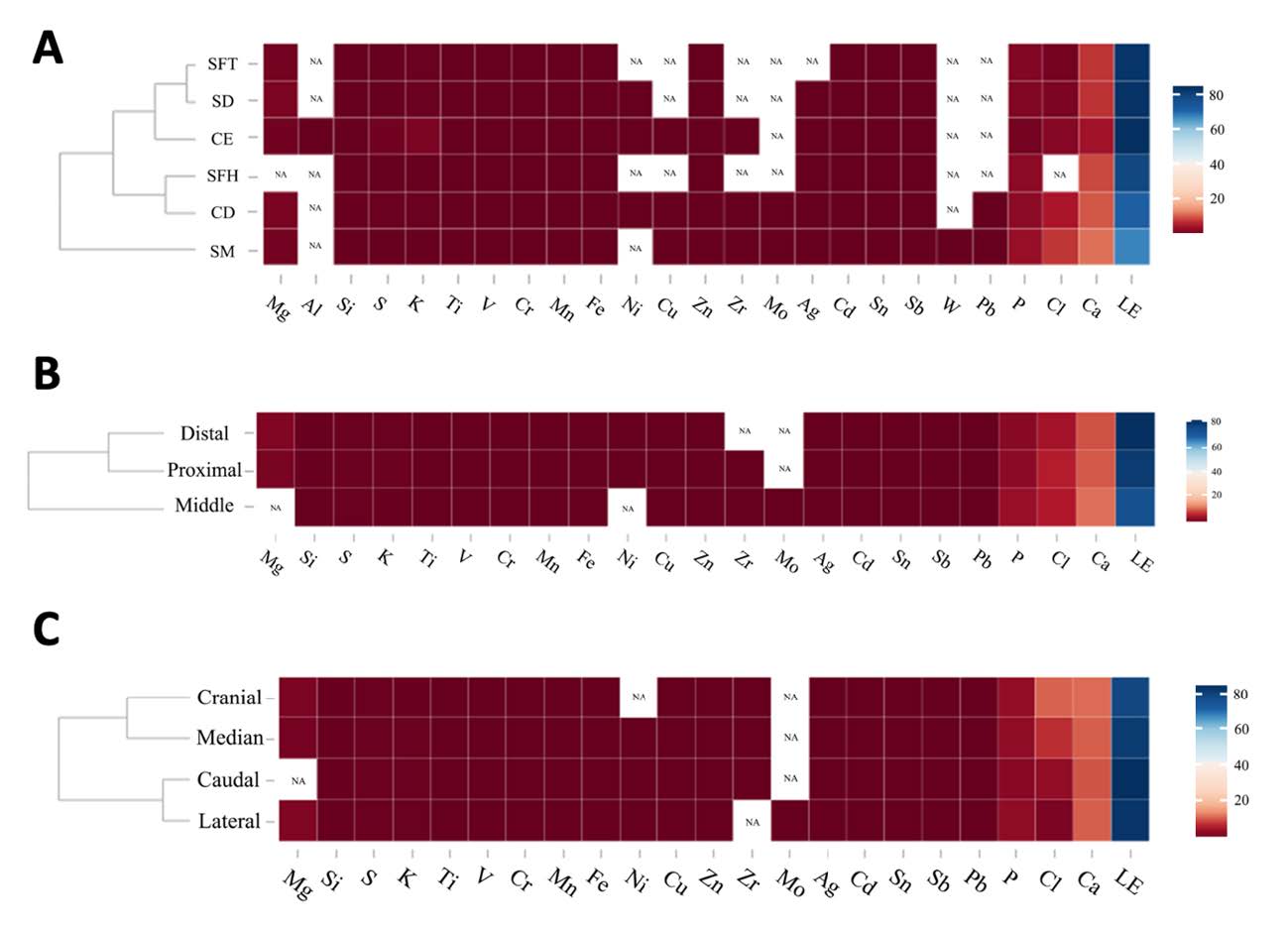
Figure 2. Clustered heat maps from mean values of the elements at 6 different locations (A), 3 different parts (B) and 4 different directions (C). The cell colors represent the percentage of elements, the highest percentage of element is blue color, while the lowest is red. CD = Compact bone at diaphysis, CE = Compact bone at epiphysis, SM = Spongy bone at metaphysis, SD = Spongy bone at diaphysis, SFT = Spongy bone at femoral trochlea, SFH = spongy bone at metaphysis. 

Stepwise discriminant analysis

          According to the stepwise discriminant analysis of different six locations in bones, it was found that the compact bone (CD and CE) had a very high accuracy rate (94.4%) (Table 4, Figure 3). Additionally, the prediction rate obtained by the spongy bone was 0%. Meanwhile, the prediction rate of the spongy bone (SM and SD) to be a compact bone (CD) was very low (5.0 and 1.8%). However, in two other category tests (Table 4, Figure 3); differences in 3 parts and 4 directions of the femoral diaphysis revealed very low accuracy rates at 63.6% and 37.0%, respectively. The numbers of the elements were 7, 4 and 1 for 6 locations, 3 parts and 4 directions, respectively (Table 5, Table 6).

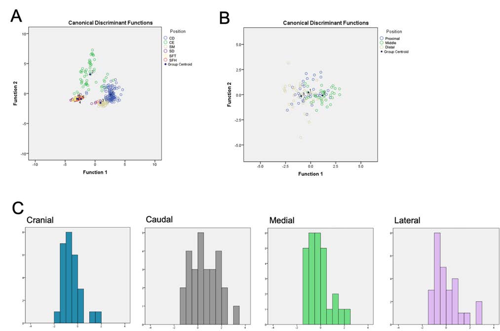
Figure 3.   Location classification achieved based on the percentage of elements using stepwise discriminant analysis. The group centroids of each species are shown in the plot. The scatter plot of the discriminant values was derived from the suitable functions of 6 different locations (A), 3 different parts (B), and 4 different directions (C). The functions 1 and 2 of each plot are indicated in Table 6. The data from 4 different directions generated one function and are present as a bar graph rather than a scatter plot. CD = Compact bone at diaphysis, CE = Compact bone at epiphysis, SM = Spongy bone at metaphysis, SD = Spongy bone at diaphysis, SFT = Spongy bone at femoral trochlea, SFH = spongy bone at metaphysis. 

Table 3.   Mean and Standard Derivation (SD) values of each element detected in compact bones at four directions of femoral diaphysis.

Note: Superscripts (a, b) indicate significant differences (P<0.05) between bone parts of the same element.

Table 4.  Classification results using the function derived from stepwise discriminant analysis to assign the parts of femoral bones.

Note:   CD = Compact bone at diaphysis, CE = Compact bone at epiphysis, SM = Spongy bone at metaphysis, SD = Spongy bone at diaphysis, SFT = Spongy bone at femoral trochlea, SFH = spongy bone at metaphysis.

Table 5. Canonical discriminant function coefficients.

Table 6. Functions at group centroids.

Note: CD = Compact bone at diaphysis, CE = Compact bone at epiphysis, SM = Spongy bone at metaphysis, SD = Spongy bone at diaphysis, SFT = Spongy bone at femoral trochlea, SFH = spongy bone at metaphysis.

DISCUSSIONS 

          Our previous studies have proposed that the elemental profile obtained from HHXRF displayed the capability of effective species classification for various species (Buddhachat et al., 2016a; Nganvongpanit et al., 2016a; Buddhachat et al., 2016b; Nganvongpanit et al., 2016b; Nganvongpanit et al., 2016c; Nganvongpanit et al., 2017a; Nganvongpanit et al., 2017b). High accuracy and precision rates were confirmed with this method. However, we also encountered many problems and/or limitations when using this method. We primarily presumed that the elemental distribution throughout a bone specimen might be heterogenous.  In this study, we needed to prove this presumption. Our findings demonstrated that the distribution of elements was considerably different between the compact and spongy bones; however, there seemed to be a homogenous distribution between the different parts of either the compact or spongy bone in the same bone pieces.

            In the compact bone, three elements were found in certain specific parts including Mg, Ni and Mo. Approximately 60% of Mg in the body was found in the bone. This involved mineral metabolism at it was indirectly identified through ATP metabolism and acted as a cofactor of many enzymes (Palacios, 2006). Nickel is an important element that serves as an ultra-trace nutrient. It is also involved in lipid metabolism and is associated with an increase in hormonal activity (Zdrojewicz et al., 2016). Molybdenum is an essential trace element for several enzymes (Zdrojewicz et al., 2016). Notably, these elements are present in very small quantities. Therefore, it is possible to find an uneven distribution of these elements in the bone. Almost all of the elements were significantly different in all parts, and the Ca/P ratio in the middle part of the diaphysis was found to be significantly lower than of the proximal and distal parts. Increasing calcification in bone tissue results in increased stress and decreased strain levels (Ascenzi et al., 2020). It is possible that the bone stress at the middle part of the diaphysis might have been lower than at the proximal and distal parts. However, in order to verify this, an additional study on the bone strength of the diaphysis parts would need to be conducted. Most of the previous studies were done by making comparisons between the distal part of the long bone (diaphysis and epiphysis) or between the compact and the spongy bones (Gdoutos et al., 1982; Raftopoulos and Qassem, 1987). Our results are in accordance with those of previous studies. It was found that the Ca/P ratio of the spongy bone was significantly lower than that of the compact bone. This indicated that the spongy bone was evidently less strong than the compact bone.

            The clustered heat map helped us to visualize the similarity of the elemental content in different ways in this study. Among the three different parts, it was found that the proximal and distal parts of the diaphysis displayed a similar degree of elemental content. It was plausible that the morphology of the bone had an effect on the elemental accumulation. The middle part of the femur or mid sharp were confirmed as both the smallest and narrowest parts, while the proximal and the distal parts of the diaphysis were similar in size but larger in the middle part. This finding was in accordance with the results from the clustering of direction, wherein the elemental content in the cranial and median parts were positioned in the same group, and the caudal and lateral were positioned in the same group. According to the anatomical position, in the standing and walking positions of four-legged animals such as in pigs, the force down to the hind-limbs is sent forward and then indented to the inside (Thorup et al., 2007; Von Wachenfelt et al., 2009). Therefore, it is possible that the amount of minerals that accumulate in the cranial and median of the femur bone were similar. The cluster of six different bone parts revealed that the spongy bone in terms of metaphysics was separated from the five other parts with regard to the anatomy. This was likely because these parts were composed of cartilage content (Dyce et al., 2009). According to the previous study, it was found that the elemental content was significantly different among different bone types: bone, cartilage and sesamoid bone (Nganvongpanit et al., 2016d). Furthermore, we tested the classification rate of each bone location via PCA. The outcome demonstrated remarkable differences in the element profile of the compact bone and the spongy bone, whereas the classification rate within the compact bone at different locations or parts did not differ significantly. Additionally, previous studies have shown that all 48 bones in dogs displayed differences in the elements present and differences in the numbers of detected elements (Nganvongpanit et al., 2016d).

CONCLUSION 

            This study has addressed an important knowledge gap in terms of the use of XRF for species classification. From the results of this study, it has been determined that with each bone piece of the same species, a few elements were found to be different between different locations. Consequently, this outcome resulted in a fairly poor classification rate. It can be concluded that the elemental distribution in each bone might not have an effect on species classification when determining the elemental composition via XRF technique.

ACKNOWLEDGEMENT 

          The authors would like to acknowledge the financial support that was provided by the Excellence Center in Veterinary Bioscience, Chiang Mai University, Thailand (2019-2020).

REFERENCES 

Ascenzi, M.G., Zonca, A., and Keyak, J.H. 2020. Effect of cortical bone micro-structure in fragility fracture patients on lamellar stress. Journal of Biomechanics. 100: 109596. https://doi.org/10.1016/j.jbiomech.2019.109596

Buddhachat, K., Brown, J.L., Thitaram, C., and Klinhom, S., Nganvongpanit, K. 2017. Distinguishing real from fake ivory products by elemental analyses: a Bayesian hybrid classification method. Forensic Science International. 272: 142-149. https://doi.org/10.1016/j.forsciint.2017.01.016

Buddhachat, K., Klinhom, S., Siengdee, P., Brown, J.L., Nomsiri, R., Kaewmong, P., Thitaram, C., Mahakkanukrauh, P., and Nganvongpanit, K. 2016a. Elemental analysis of bone, teeth, horn and antler in different animal species using non-invasive handheld X-ray fluorescence. PLoS One 11: e0155458. https://doi.org/10.1371/journal.pone.0155458

Buddhachat, K., Piboon, P., and Nganvongpanit, K. 2019. Effect of lacquer on altered elemental proportions in the superficial layer of bone, using handheld X-ray fluorescence. Songklanakarin Journal of Science and Technology. 41: 700-707.

Buddhachat, K., Thitaram, C., Brown, J.L., Klinhom, S., Bansiddhi, P., Penchart, K., Ouitavon, K., Sriaksorn, K., Pa-in, C., Kanchanasaka, B., et al. 2016b. Use of handheld X-ray fluorescence as a non-invasive method to distinguish between Asian and African elephant tusks. Scientific Reports. 6: 24845. https://doi.org/10.1038/srep24845

Castro, W., Hoogewerff, J., Latkoczy, C., and Almirall, J.R. 2010. Application of laser ablation (LA-ICP-SF-MS) for the elemental analysis of bone and teeth samples for discrimination purposes. Forensic Science International. 195(1-3): 17-27. https://doi.org/10.1016/j.forsciint.2009.10.029

Corrieri, B., and Márquez-Grant, N. 2019. Using nutrient foramina to differentiate human from non-human long bone fragments in bioarchaeology and forensic anthropology. Homo. 70(4): 255-268. https://doi.org/10.1127/homo/2019/1113

Cortellini, V., Carobbio, A., Brescia, G., Cerri, N., and Verzeletti, A. 2019. A comparative study of human and animal hairs: Microscopic hair comparison and cytochrome c oxidase I species identification. Journal of Forensic Science and Medicine. 5: 20-23.

Cummaudo, M., Cappella, A., Biraghi, M., Raffone, C., Màrquez-Grant, N., and Cattaneo, C. 2018. Histomorphological analysis of the variability of the human skeleton: forensic implications. International Academy of Legal Medicine. 132(5): 1493-1503. https://doi.org/10.1007/s00414-018-1781-0

Cummaudo, M., Cappella, A., Giacomini, F., Raffone, C., Màrquez-Grant, N., Cattaneo, C. 2019. Histomorphometric analysis of osteocyte lacunae in human and pig: exploring its potential for species discrimination. International Academy of Legal Medicine. 133(3): 711-718. https://doi.org/ 10.1007/s00414-018-01989-9

Dyce, K.M., Sack, W.O., and Wensing, C.J.G. 2009. Textbook of veterinary anatomy. 4^th ed. Philadelphia: Saunders. 848 p.

Engle, S., Whalen, S., Joshi, A., and Pollard, K.S., 2017. Unboxing cluster heatmaps. BMC Bioinformatics. 18: 63.

Gdoutos, E.E., Raftopoulos, D.D., and Baril, J.D. 1982. A critical review of the biomechanical stress analysis of the human femur. Biomaterials. 3(1): 2-8. https://doi.org/10.1016/0142-9612(82)90053-9

Holland, M.M., and Parsons, T.J. 1999. Mitochondrial DNA sequence analysis - validation and use for forensic casework. Forensic Science Review. 11:
21-50.

Moore, M.K., and Frazier, K. 2019. Humans are animals, too: critical commonalities and differences between human and wildlife forensic genetics. Journal of Forensic Sciences. 64(6): 1603-1621. https://doi.org/
10.1111/1556-4029.14066

Nganvongpanit, K., Brown, J.L., Buddhachat, K., Somgird, C., and Thitaram, C. 2016a. Elemental analysis of Asian elephant (Elephas maximus) teeth using X-ray fluorescence and a comparison to other species. Biological Trace Element Research. 170(1): 94-105. https://doi.org/10.1007/s12011-015-0445-x

Nganvongpanit, K., Buddhachat, K., Brown, J.L., Klinhom, S., Pitakarnnop, T., and Mahakkanukrauh, P. 2016b. Preliminary study to test the feasibility of sex identification of human (Homo sapiens) bones based on differences in elemental profiles determined by handheld X-ray fluorescence. Biological Trace Element Research. 173(1): 21-29. https://doi.org/10.1007/s12011-016-0625-3

Nganvongpanit, K., Buddhachat, K., Klinhom, S., Kaewmong, P., Thitaram, C., and Mahakkanukrauh, P. 2016c. Determining comparative elemental profile using handheld X-ray fluorescence in humans, elephants, dogs, and dolphins: preliminary study for species identification. Forensic Science International. 263: 101-106. https://doi.org/10.1016/j.forsciint.2016.03.056

Nganvongpanit, K., Buddhachat, K., Piboon, P., Euppayo, T., Kaewmong, P., and Cherdsukjai, P., Kittiwatanawong, K., Thitaram, C. 2017a. Elemental classification of the tusks of dugong (Dugong dugong) by HH-XRF analysis and comparison with other species. Scientific Reports. 7: 46167. https://doi.org/10.1038/srep4616

Nganvongpanit, K., Buddhachat, K., Piboon, P., Euppayo, T., and Mahakkanukrauh, P. 2017b. Variation in elemental composition of human teeth and its application for feasible species identification. Forensic Science International. 271: 33-42. https://doi.org/10.1016/j.forsciint.2016.12.017

Nganvongpanit, K., Buddhachat, K., Piboon, P., and Klinhom, S. 2016d. The distribution of elements in 48 canine compact bone types using handheld X-ray fluorescence. Biological Trace Element Research. 174: 93-104. https://doi.org/10.1007/s12011-016-0698-z

Nganvongpanit, K., Kaewkumpai, P., Kochagul, V., Pringproa, K., Punyapornwithaya, V., and Mekchay, S. 2020. Distribution of melanin pigmentation in 32 organs of Thai black-bone chickens (Gallus gallus domesticus). Animals. 10(5):  777. https://doi.org/10.3390/ani10050777

Nganvongpanit, K., Phatsara, M., Settakorn, J., and Mahakkanukrauh, P. 2015. Differences in compact bone tissue microscopic structure between adult humans (Homo sapiens) and Assam macaques (Macaca assamensis). Forensic Science International. 254: 243.e1-243.e5. https://doi.org/10.1016/j.forsciint.2015.06.018

Palacios, C. 2006. The role of nutients in bone health, from A to Z. Critical Reviews in Food Science and Nutrition. 46. https://doi.org/10.1080/
10408390500466174

Pereira, F., Alves, C., Couto, C., Díaz, L.L., Parra, D., Furfuro, S., Aler, M., Borrego, L.B., Olekšáková, T., Balsa, F., et al. 2019. Species identification in routine casework samples using the SPInDel kit. Forensic Science International: Genetics Supplement Series. 7: 180-181. https://doi.org/10.1016/j.fsigss.2019.09.070

Raftopoulos, D.D., and Qassem, W. 1987. Three-dimensional curved beam stress analysis of the human femur. Journal of Biomedical Engineering. 9(4): 356-366. https://doi.org/10.1016/0141-5425(87)90085-9

Ryan, M.C., Stucky, M., Wakefield, C., Melott, J.M., Akbani, R., Weinstein, J.N., and Broom, B.M. 2020. Interactive clustered heat map builder: an easy web-based tool for creating sophisticated clustered heat maps [version 2; peer review: 2 approved]. International Society for Computational Biology Community Journal. 8: 1750. https://doi.org/10.12688/f1000research.20590.2

Schotsmans, E.M.J., Marquez-Grant, N., Forbes, S.L. 2017. Taphonomy of human remains: forensic analysis of the dead and the  depositional environment. Hoboken, New Jersey: John Wiley & Sons.

Thorup, V.M., Tøgersen, F.A., Jørgensen, B., and Jensen, B.R. 2007. Biomechanical gait analysis of pigs walking on solid concrete floor. Animal. 1: 708-715.  https://doi.org/10.1017/S1751731107736753

Von Wachenfelt, H., Pinzke, S., Nilsson, C., Olsson, O., and Ehlorsson, C.J. 2009. Force analysis of unprovoked pig gait on clean and fouled concrete surfaces. Biosystems Engineering. 104(2): 250-257. https://doi.org/10.1016/j.biosystemseng.2009.06.010

Zdrojewicz, Z., Popowicz, E., and Winiarski, J. 2016. Nickel - role in human organism and toxic effects. Polskiego Towarzystwa Lekarskiego. 41: 115-118. https://doi.org/10.1016/j.biosystemseng.2009.06.010