ABSTRACT

With a conventional NMR (Nuclear Magnetic Resonance) spectrometer, the study sample is placed inside the magnet. In contrast, with a single-sided NMR spectrometer, the study sample is outside, but close to the magnet. Singlesided spectrometers can thus be used with a large sample and made portable. A high magnetic field can be achieved without the need for a high-current, DC power supply when using neodymium (NdFeB) magnets. The system is, therefore, relatively low cost, as well.

The U-shaped magnet developed here consists of two permanent magnets of size 50x50x25 mm³ (with a measured surface magnetic field of 0.35 T) placed on a piece of thick steel with opposite poles upward, giving a magnetic field parallel to the surface of the magnets. The magnetic charge model was used to calculate the magnetic field in planes at different distances from the magnets’ surface and the size of the NMR sensitive region with 103 ppm homogeneity was obtained. Calculated field values and values measured using a tesla meter allowed the values of the surface magnetic charge density σ_m to be determined. Magnets positioned with a gap of one-half the width of the magnet face produced the largest sensitive region. In this case, the sensitive region was 12 x 2.5 x 1 mm and located 15 mm above the magnet surface with a central field of 0.23 T.

Keywords: Single-sided NMR, Mobile NMR, NMR spectrometers, U-shaped magnet, Magnetic charge model

INTRODUCTION

Nuclear Magnetic Resonance (NMR) is a phenomenon whereby a nucleus with non-zero spin, and thus a magnetic moment, will absorb energy from an irradiating electromagnetic wave when placed in an external static magnetic field (B₀). The specific frequency absorbed, known as the Larmor frequency (f₀), is given by the simple relationship (f₀ = γB₀/2π (Levitt, 2001). The constant γ is the gyromagnetic ratio for that particular nucleus. For example, a hydrogen nucleus (¹H) or proton will resonate at 42.578 MHz in a field of 1 T. Experimentally, the radio frequency (RF) wave is applied by an RF-coil with its magnetic field component (B₁) perpendicular to the main field B₀. NMR has been applied in many fields including chemistry, physics, medicine and engineering as well as in the chemical industries (Blumich et al., 2008).

An NMR spectrometer consists of a magnet, a transmitter, a receiver and software (Levitt, 2001). As each part is complicated, expensive and large, NMR spectrometers are typically found only in hospitals and large laboratories.

NMR spectrometer magnets have been developed in various forms, but normally the object under study is placed inside an RF-coil situated in the core/gap of the magnet. However, in a single-sided magnet NMR spectrometer (Blumich et al., 2008), such as the NMR-MOUSE (Mobile Universal Surface Explorer) (Eidmann et al., 1996, Blumich et al., 1998, Goga et al., 2006), the object to be measured is placed outside the RF-coil and magnet, in a sensitive region where the Larmor condition is satisfied. A single-sided NMR magnet normally consists of two pieces of permanent magnet embedded in an iron yoke (Eidmann et al., 1996) or placed on a piece of thick steel with anti-parallel magnetization (Goga et al., 2006). The RF coil is positioned either inside the gap or slightly above the gap between the two permanent magnets, so that the static magnetic field B₀ and the RF field B₁ are approximately orthogonal to each other within a sensitive region above the magnet surface (Blumich et al., 2008).

The single-sided NMR spectrometer offers several advantages:  

• mobility, due to its small size,

• the ability to image large samples, given the NMR-sensitive region is outside the magnets (Blumich et al., 2008) and,

• achievement of a high magnetic field without the need for a high-current, DC power supply.

Single-sided NMR spectrometers have been used in applications such as analyzing the structure of chemicals, the detection of moisture in soil, concrete bridge decks and building materials, food quality and product control, medical diagnostics and on-line monitoring (Blumich et al., 2008).

In this work, we placed two rectangular neodymium (NdFeB) permanent magnets of size 50x50x25 mm³ (with a magnetic field of 0.35T at the surface of the magnets) with opposite polarization on a piece of thick steel to give a U-shaped permanent magnet (Figure1). The magnetic charge model (Furlani, 2001) was used to calculate the magnetic field in the plane at different distances from the magnet surface. The field was also measured experimentally using a Tesla meter (Phywe, Germany) with an error of ± 0.5% (± 1 mT). The gap between magnets was varied to find the best positioning for creating a large sensitive region.

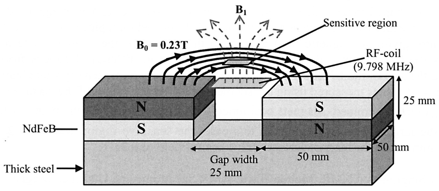
Figure 1. Principle of the one-sided magnet: The static magnetic field B₀ and the RF field B₁ are approximately orthogonal to each other in the sensitive region.

MATERIALS AND METHODS

In this section, we describe a method for analyzing permanent magnets using the magnetic charge model, and then find an expression for the magnetic field at any point outside the rectangular permanent magnet. The best set-up for the U-shaped magnet was found by an optimization process.

The charge model

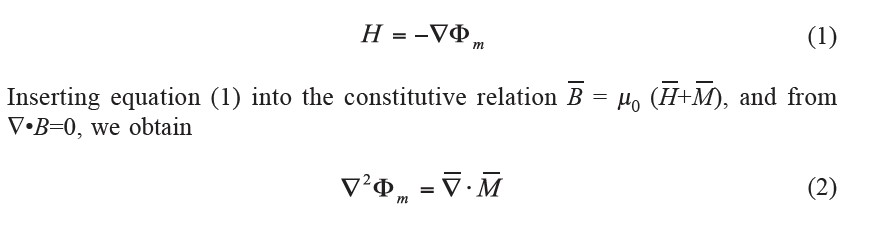
In general, two main methods are used for calculating the magnetic field produced by a permanent magnet (Jackson, 1999): magnetic scalar potential, which uses effective magnetic charge density; and vector potential, which uses effective magnetic current density. Furlani (2001) demonstrated that both methods give the same result under the charge and current models. Since current density is a vector, when integrating, the direction of the current density has to be taken into consideration. In contrast, charge is scalar, with no directional component involved. As the charge model is simpler, it was chosen for field calculation in this study. The “magnetic charge” density distribution is used as a source term in the magnetostatic field equations and the fields are obtained using standard methods. From Maxwell’s equations, the magnetostatic equations for the current free regions are ∇ × H = 0 A/m² and ∇•B = 0 Wb/m³. Since the curl of a gradient of a scalar function is zero, the former equation implies that we can introduce a magnetic scalar potential Φ_m (Jackson, 1999) such that,

Equation (2) becomes a magnetostatic Poisson equation   where is the effective magnetic charge density with

Similar to the electrostatic field case, the solution for the magnetic scalar potential Φ_m when there are no boundary surfaces is:

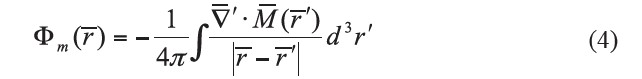
where  is the observation point or field point,   is the source point, and operates on the primed coordinates of the source. If the magnetization   is limited to a volume V and assumed to fall to zero at the surface S, then equation (4) becomes (Jackson, 1999, chapter 5)

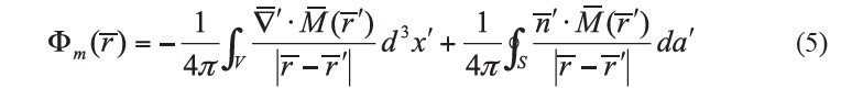
where S is the surface that bounds V and  n' is the outward normal unit vector to the surface S. Application of the divergence theorem to  (Jackson, 1999) in a Gaussian pillbox straddling the surface shows that there is an effective magnetic surface charge density  of

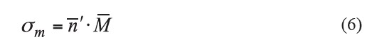
If the permanent magnet is in free space at a field point external to the magnet of  and if the magnetization  is assumed to be constant in the volume V, then the effective magnetic charge density  is zero. We find that (Furlani, 2001),

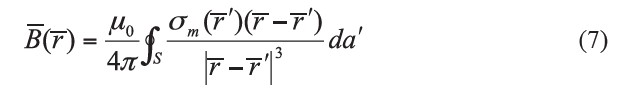
The equation (7) is used to calculate the magnetic field of a rectangular bar permanent magnet in the next section.

Rectangular structures

Using the charge model method and equation 7, we can calculate the magnetic field  of a rectangular bar permanent magnet which has a bipolar magnetization pattern. We can reduce the magnet to an equivalent charge distribution at its two poles as shown in Figure 2. If the magnetization  is assumed to be constant, has the value M_s and is in the z direction, then from equation (3) the volume charge density becomes zero, i.e.  Thus, only the magnetic surface charge density at the poles needs to be taken into account. From equation (6), , we have  for the top surface (z = z₂) and for the bottom surface (z = z₁) of the magnet.

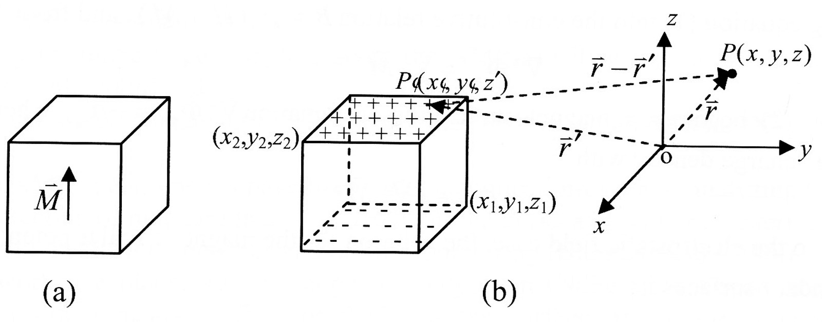
Figure 2. Rectangular bar permanent magnet: (a) physical magnet with assumed uniform magnetization, (b) equivalent surface charges and coordinates of the observation point P(x,y,z) and the source point 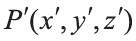 used in calculation.

From equation (7) and Figure 2, we can find the y component of the magnetic field B y (x,y,z) at any point outside the rectangular bar permanent magnet from

Calculation and experimental design

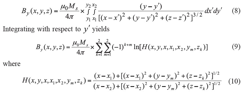
The U-shaped permanent magnet design is shown in Figure 3. The magnetic field is in a direction parallel to the surface of the magnets along the y-axis. In the calculation, the origin of coordinates is set at the top center of the gap between the magnets as shown in Figure 3. The magnet gap was varied over 10, 15, 20, 25 and 30 mm. The distance along the z-axis above the magnet surface was set at distances of 3, 5, 10, 15, 20, 25, 30, 35 and 40 mm. The steps used in calculation of the magnetic field in the x and y directions was 0.25 mm. Equation (9) was then used to calculate the magnetic field B_y along the x- and y-axes to find the best positions for the magnets in terms of magnetic field and field uniformity.

Experimental measurements were performed using a Tesla meter (Phywe, Germany). The measurement conditions were similar to the calculation conditions, with the difference that the measurement step in the x- and y-axis used was 2.5 mm. Calculations and measurements were used to choose the best gap width between the magnets.

Figure 3. U-shaped permanent magnet and the coordinate system used.

In order to determine the surface charge density  needed for the calculation, the measurement data were compared with the calculation results point-bypoint to find an average . This value for  was substituted back into equation (9) and the magnetic field was recalculated. To find the best gap, the level of homogeneity of magnetic field U was determined using the homogeneity condition , where B is the calculated magnetic field value, B₀ the magnetic field value at the middle of the gap and U is in parts per million (ppm). We selected the best sensitive region over distances of 3 to 40 mm along the z-axis.

RESULTS

The comparison between the calculated field values and the measured field values produced an average value of the surface magnetic charge density  of 1.33x105 A/m. Figure 4 shows the results of the measurement (a, c) and calculation (b, d) of the magnetic field B_y along the y- and x- axes, respectively, at different heights above the magnet surface for the chosen best magnet gap of 25 mm. These results indicate that the distance above the magnet surface where the field is reasonably homogeneous is at z = 15 mm, with a central field of 230 mT. The value for the best magnet gap was determined from a plot of the size of the sensitive region along the y axis for different homogeneity U values in the plane z = 15 mm above the magnet surface for different magnet gaps as shown in Figure 4 (e). As can be seen from this figure, the best sensitive region along the y axis for field homogeneity tolerance of U = 10³ ppm is when the gap is 25 mm, which results in a sensitive region of 12 mm in the y direction. Similar calculations in the x direction gave 2.5 mm and in the z direction gave 1 mm, which are much smaller than in the y direction. Thus, the sensitive region in the middle of the gap at 15 mm above the top magnet surface for field homogeneity within 10³ ppm is in the region of x = ±1.25 mm, y = ±6.0 mm and z = 15±0.5 mm for the magnet gap of 25 mm. Here, the magnetic field in the y direction varies at most ±0.23 mT from the value of 230 mT at the center of the region.

Figure 4. Measured (a, c) and calculated (b, d) magnetic field B_y on the y axis (a, b) and on the x axis (c, d) at different heights above the magnet surface with a magnet gap of 25 mm. (e) Width of sensitive region in the y direction in the plane z = 15 mm for different ppm values of field homogeneity tolerances with different magnet gaps. 

DISCUSSION

The size of the sensitive region at 15mm above the magnet surface as found from Figure 4 is much greater in y than in x and z. In order to increase the size of the sensitive region, the plane of the sensitive region must be further away from to the magnet surface. However, this results in an undesired decrease in the magnetic field intensity. One way to increase the sensitive region size in the x direction is to increase the size of the magnet in the x direction. The size of the sensitive region depends on the size of the permanent magnets, the gap width between the magnets, the required magnetic field intensity and the level of field homogeneity. The further one goes away from the top of the magnet the larger the sensitive region with field intensity being sacrificed. For a larger sensitive region such as for NMR imaging (MRI), either larger magnets or additional smaller magnets are required, as well as magnetic field shimming in order to increase field homogeneity (Goga et al., 2006).

Another factor that affects the size and shape of the sensitive region is the shape of the magnet. Eidmann et al. (1996) used two semi-cylindrical shaped NdFeB permanent magnets (0.5 T at the magnet surface) of 31 mm in height and 55 mm in diameter embedded in an iron yoke and placed face-to-face with antiparallel magnetization. This gave a magnetic field parallel to the plane surface of the magnets. The shape of the sensitive region is ellipsoidal and the width of the sensitive region is governed by the width of the gap between the magnets (Blumich et al., 1998).

Comparison between calculated field values and measured values allows the surface magnetic charge density to be determined. The best set-up occurred when the gap between the magnets was one-half the width of the magnet in the direction perpendicular to (across) the gap. This finding is similar to that shown in the principle of the NMR-MOUSE (Figure 1 in Blumich et al., 1998), which used a gap of 13 mm between 2 rectangular magnets of width 26 mm and height 32 mm (length not shown). For a U-shaped magnet made from two rectangular NdFeB permanent magnets of square cross section (50 mm wide and 25 mm high) with measured surface field intensity of 350 mT and a gap of 25 mm between the magnets, the obtained sensitive region of homogeneity (10³ ppm at 15 mm above the top surface gap of the magnet) is of size:

• 12 mm in the direction across the gap,

• 2.5 mm in the direction along the gap and

• 1 mm thick.

Within this sensitive volume, the magnetic field in the direction across the gap has variation of 0.23 mT from the value of 230 mT at the centre of the region. Improvement to increase the region of field homogeneity along the gap could be made by increasing the size of the magnet in that direction.

The results of this paper establish the best set-up for a U-shaped permanent magnet for a single-sided spectrometer with a relatively large sensitive region above the gap between the magnets at a specified distance above the magnet surface. The result can be used to construct a single-sided U-shaped magnet from two rectangular magnets and a NMR surface coil can be designed to sense the NMR signal from this sensitive region inside the study sample. Knowing the field distribution inside the sensitive region will allow design for magnetic field shimming to improve the field homogeneity. The link between the magnet geometry and the sensitive region shape and size found in this work suggests future work on optimization of magnet system design for a particular sensitive region, as well as the possibility of making use of the “built in” magnetic gradient in the direction away from the pole faces for magnetic resonance imaging.

ACKNOWLEDGEMENTS

This project was funded by the Development and Promotion of Science and Technology Talents Project (DPST), the National Research Council of Thailand (NRCT) and Department of Physics, Khon Kaen University.

REFERENCES

Blumich B., P. Blumler, G. Eidmann, A. Guthausen, R. Haken, U. Schmitz, K. Saito, and G. Zimmer. 1998. The NMR-MOUSE: construction, excitation, and applications. Magnetic Resonance Imaging, 16:479-484. 10.1016/S0730-725X(98)00069-1

Blumich B., J. Perlo, and F. Casanova. 2008. Mobile single-sided NMR. Progress in Nuclear Magnetic Resonance Spectroscopy, 52: 197-269. 10.1016/j.pnmrs.2007.10.002

Eidmann G., R. Savelsberg, P. Blumler, and B. Blumich. 1996. The NMR MOUSE: a mobile universal surface explorer. Journal of Magnetic Resonance, A122: 104-109.

Furlani E.P. 2001. Permanent Magnet and Electromechanical Devices. New York: Academic Press; pp.126-135, 208-217.

Goga N.O., A. Pirnau, L. Szabo, R. Smeets, D. Riediger, O. Cozar, and B. Blümich. 2006. Mobile NMR: applications to materials and biomedicine. Journal of Optoelectronics and Advanced Materials, 4: 1430-1434.

Jackson J.D. 1999. Classical Electrodynamics. 3rd ed. New York: John Wiley & Sons; pp.194-197.

Levitt M.H. 2001. Spin Dynamics Basics of Nuclear Magnetic Resonance. Chichester, England: John Wiley & Sons; pp.5-15.