ABSTRACT

In this study, we examined monthly temperature variation from 1973 to 2008 on grid regions of the earth surface above latitude 45°North, covering the Arctic Ocean, northern areas of the Atlantic and Pacific Oceans, and the Asian and European continent. Linear modelling was used to investigate the trends and patterns of temperature changes and account for auto-correlations of the temperature changes over time. Factor analysis was then used to model filtered residuals, i.e., the residuals after removing time trends and auto-correlation, providing a basis for identifying and classifying regions with similar temperature change. Twelve large regions, each having similar temperature change patterns, were identified. Of the 69 sub-regions considered in the study, 64 sub-regions experienced significant increase in temperature, 2 sub- regions had insufficient data, and only 3 sub-regions remained unchanged. High temperature increases (0.200°C to 0.320°C) occurred in the North Pacific Ocean, Alaska and Eastern Siberia. Moderate temperature increases (0.130°C to 0.199°C) occurred in north Canada, Greenland, Iceland, Norway, Sweden and Finland. The north of Siberia and part of the North Atlantic had low increases (0.090°C to 0.129°C) while northeast Canada and its surrounding seas did not show evidence of warming.

Keywords: Latitude, Climate change, Time series analysis, Correlation, Auto-correlation, Factor analysis.

INTRODUCTION

Earth surface temperature change is one of the most important issues the world faces today. Global surface temperature has changed over the past 150 years, with a slightly higher rate of warming in the 20th century (Jones et al., 1999). This warming is associated with change in sea levels, destruction of ecosystems, shrinkage of mountain glaciers, reduction of ice cover (National Academies Report, 2008) and altered ocean circulation patterns (Houghton et al., 2001).

Increased surface temperature in the Arctic Ocean has been a major topic of international reviews and indigenous observations during the last decade (Krupnik and Jolly, 2012). According to the study by Overpeck et al. (1997), the average temperature in the Arctic increased about 0.6°C from the beginning of the 20^th century and the maximum temperatures there have increased approximately 1.2°C since 1945. The temperature change was about +1°C per decade (increase) in the eastern Arctic Ocean and -1°C per decade (decrease) in the western Arctic Ocean during the winter season. Furthermore, significant warming in spring has been detected across most of the Arctic region (Rigor et al., 1999).

Various studies have assessed temperature changes over the Earth’s surface. For example, Box et al. (2007) studied temperature changes in Greenland over the period 1840-2007. The annual warming trend in 1919-1932 was 33% greater than in 1994-2007, and the recent warming was high in western Greenland during autumn and southern Greenland in winter. In addition, Anisimov et al. (2007) investigated the changes of air temperature in Russia over the period 1900-2004. The trend of the annual average temperature was 0.5°C per 100 years in the north of European Russia and 1.4°C-1.6°C per 100 years in the south of Ural Siberia and the Far East. On average for the entire territory of Russia, the trend was 1.1°C per 100 years.

It is not easy to understand and explain the variability and trends of change in Earth surface temperatures or quantify the size and speed of the rate of change. Many scientists and researchers have studied patterns of Earth surface temperature changes in different regions of the world using various methodologies, including computer simulation models (Johannessen et al., 2003), empirical orthogonal functions (Semenov, 2007) and statistical techniques, such as multiple linear regression (Lean and Rind, 2009), multiple regression with non-Gaussian correlated errors and linear autoregressive moving average (ARMA) model (Hughes et al., 2006) and linear spline functions and factor analysis (McNeil and Chooprateep, 2013). A more recent study by McNeil and Chooprateep (2013) investigated temperature changes in a region covering the northern Atlantic Ocean. The present study examines the region centered around the middle part of the Northern hemisphere of the Earth’s surface for temperature changes, using a combination of statistical techniques, including linear regression allowing for auto-correlation (Venables and Ripley, 2002) and factor analysis (Johnson, 1998). We examined and quantified the trend and patterns of the temperature changes across the Earth surface above 45 degrees north from 1973 to 2008, based on monthly temperature data. The area studied includes both land and sea.

MATERIALS AND METHODS

Temperature data from 1973 to 2008 for the study area were obtained from the Climatic Research Unit at the University of East Anglia, UK (CRU, 2009). They include 432 monthly average temperature anomalies (defined as excesses over monthly averages for 1961-1990; CRU, 2009) for all 5° by 5° latitude-longitude grid-boxes on the Earth’s surface studied, and were collected from weather stations, ships and, more recently, satellites. This area comprises 648 5° by 5°grid-boxes above latitude 45 degrees North, including the Arctic Ocean, the northern areas of the Atlantic and Pacific Oceans, and the North American, Asian and European continents. However temperature data were missing in a number of those grid-boxes, particularly in the polar zones. Therefore, the 648 grid-boxes were combined into 69 sub-regions of similar size (approximately 0.45 km2) for each region, following a design in the shape of an igloo. These 69 sub-regions include one covering up to 5° below the North Pole (85°N-90°N), eight in the 75°N-85°N band, 12 in the 65°N-75°N band, 24 in the 55°N-65°N band and another 24 in the 45°N-55°N band (Figure 1). A number of those sub-regions have missing data, as shown in brackets in Figure 1.

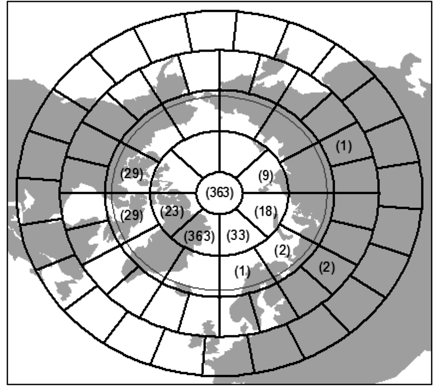
Figure 1. Map of the 69 sub-regions above latitude 45 degrees North. Numbers in brackets are the number of months with missing data for 1973-2008.

Statistical methods

A separate linear regression model was first fitted to the average monthly temperature anomalies for each of the 69 sub-regions. The model takes the following form:  

y_it = b_0i + b_1it + ∈_it for i = 1,2,...,69 and t = 1,2,...,432              (1)

where y_it denotes the average monthly temperature anomaly in sub-region i for month, corresponds to the temperature anomaly change per month in sub-region i, b_0i is the intercept (not of direct interest to our study) and ∈_it is the error assumed to follow a normal distribution with constant variance.

Residuals (y_it) from the linear model (1) were analyzed using an autoregressive model AR(2). Filtered average monthly temperature anomalies (z_it) were then obtained by removing auto-correlations at lags 1 and 2 months using the equation (Chatfield, 1996) as follows:

In these equations, y_it is the difference between the average monthly temperature anomaly in sub-regions i for month t(y_it) and the corresponding fitted value (ŷ_it), z_it is the filtered average monthly temperature anomaly in sub-region i at month, and a1, a2 are the average coefficients of the fitted auto-regressive models AR(2) across all 69 sub-regions.

Factor analysis (Johnson, 1998) was used to model the filtered average monthly temperature anomalies of the 67 sub-regions, not including the two sub-regions with insufficient data (see Figure 2 in next section), having 84% data missing. The factor analysis model with m factors (m < 67), denoted by f1, f2, ..., f_m, takes the form:

where z_it is the filtered average monthly temperature anomaly in sub-region i at month t, µ_i is the average across 432 months for sub-region i, λ_ik is the factor loadings at the i^th sub-region on the k^th factor and f_k is the k^th common factor.

As a result, inter-correlated sub-regions among the 67 sub-regions were identified. The highest inter-correlated sub-regions, i.e., those with similar filtered average monthly temperature anomalies, were classified and regrouped to form a larger region (factor) by maximizing the likelihood of the covariance matrix and minimizing the correlation between the factors for a specified number of factors, which needed to be specified in advance. The loadings (usually between -1 and 1) were controlled by rotating the factors, using the Promax method, to make these loadings as close as possible to 0 or 1. Ideally, each variable (i.e., a sub-region in our data) is correlated with only one factor, so that the correlation matrix of the residuals from this model is close to a diagonal matrix. For each of the large regions identified in the factor analysis, change in (filtered) temperature was estimated by fitting a linear model. All analyses and graphical displays were carried out using R (R Development Core Team, 2009).

RESULTS

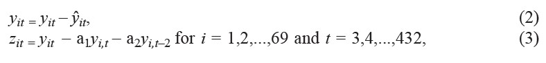
Based on the estimated temperature change per month, obtained from the simple linear regression of time for each of the 69 sub-regions, temperature change per decade was derived and mapped in Figure 2, where red represents a significant increase (p-value < 0.05), orange no evidence of change and white insufficient data in the sub-region. Of the 69 sub-regions, average monthly temperature increased in all but five sub-regions. There is no evidence of change in three and insufficient data in two of these five sub-regions. The two sub regions with insufficient data were omitted in further analysis.

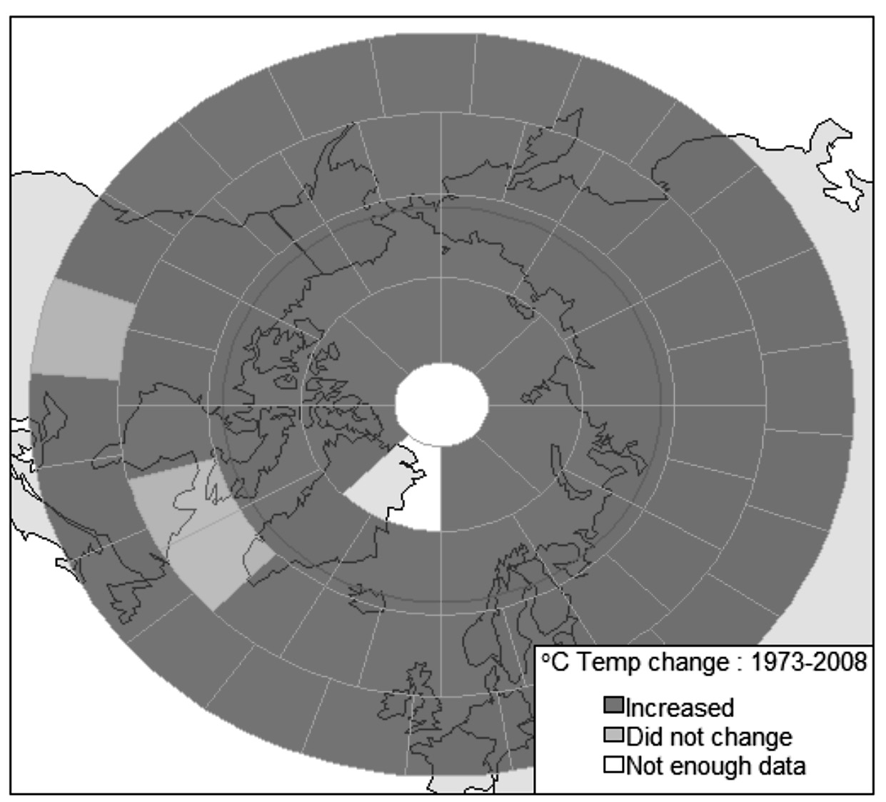
Figure 2. Map of temperature changes of the 69 sub-regions from 1973 to 2008 (before removing auto-correlations).

The time series plots of the three sub-regions that had no evidence of temperature change from 1973 to 2008 are presented in Figure 3. These sub-regions were latitude 55°N–65°N longitude 135°W–120°W (p-value = 0.116), latitude 55°N–65°N longitude 120°W–105°W (p-value = 0.065) and latitude 45°N–55°N longitude 85°W–70°W (p-value = 0.764).

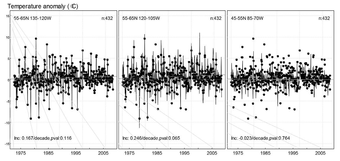
Figure 3. The time series plot of filtered average monthly temperatures anomalies in the three sub-regions with no evidence of change.

The 95% confidence intervals of temperature change per decade for each of the 67 sub-regions were estimated and plotted in Figure 4, ordered by latitude N and longitude from 180 W. A 95% confidence interval covering zero implies no significant temperature change. It confirms the results shown in Figures 2 and 3.

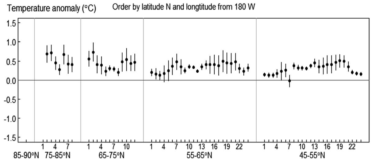
Figure 4. 95% confidence intervals of monthly temperature anomalies changes, ordered by latitude N and longitude from 180W. The horizontal axis shows sub-regions in each group of latitudes.

Residuals after removing a time trend for each region were used to assess possible auto-correlations over time. These residual time series are assumed to be stationary. Figure 5 is a graph of auto-correlation functions (ACF) of the residuals for two of the 67 sub-regions. Coefficients a1 and a2 were obtained by fitting an auto-regressive model with two parameters to the data in each region.

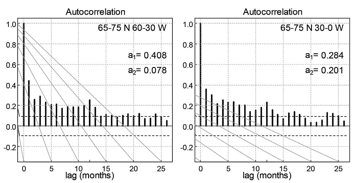
Figure 5. Auto-correlation function plots of the residuals for two of the 67subregions. The dotted line represents the 95% confidence interval of a zero correlation.

The average coefficients, and of the fitted auto-regressive models AR(2) across all the 67 sub-regions, are 0.333 and 0.04, respectively. Filtered residuals were then obtained after removing the auto-correlation structure using those average coefficients. Figure 6 contains the ACF plots of the filtered residuals for the same two of the 67 sub-regions illustrated in Figure 5. It shows that those filtering residuals are reasonably free of any auto-correlation.

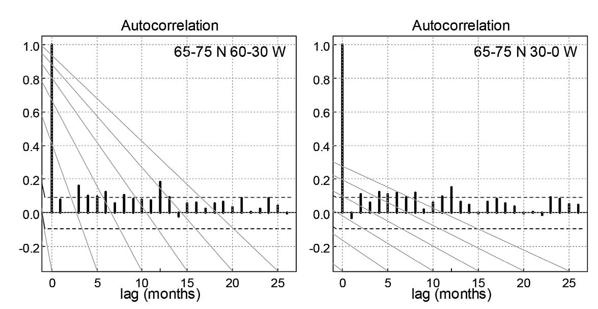
Figure 6. Auto-correlation function plots of the filtered residuals for the two sub-regions illustrated in Figure5. The dotted line represents the 95% confidence interval for a zero correlation.

Factor analysis of those filtered residuals was applied to the 67 sub-regions and resulted in 12 factors. Each factor with a unique pattern of temperature change represents a large region that consists of two to nine adjoining sub-regions (coded from 1 to 12 in Figure 7). Five (in cream in Figure 7) of the 67 sub-regions included in the factor analysis had high uniqueness.

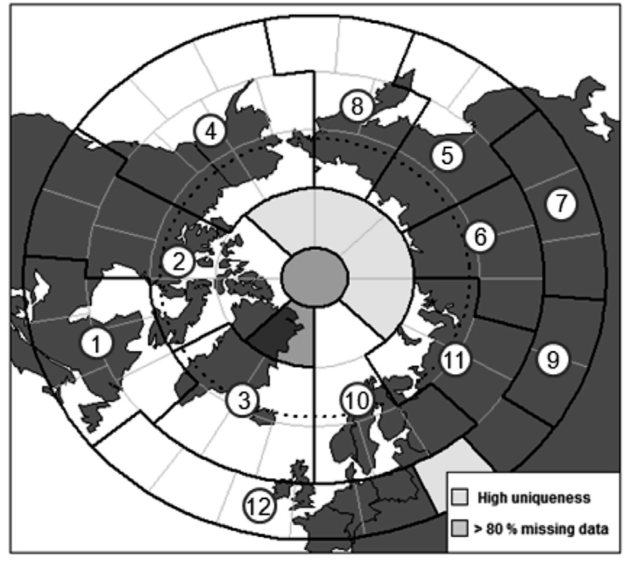
Figure 7. Twelve large regions (coded 1-12) identified from factor analysis.

The correlation matrix of the filtered residuals between pairs of the sub-regions within each of the 12 large regions is displayed as dots in the left panel of Figure 8. It is clear that sub-regions within each large region are highly positively correlated (showing large black dots) with each other, but there is little correlation (small faded dots) between pair of sub-regions from different large regions. The circles in the right panel of Figure 8 is based on residuals derived from the factor model, which shows very little correlation between pairs of sub regions even within the same large region, as expected. This indicates that the factor model has largely accounted for the correlation between those sub-regions considered, suggesting that the 12 factors explain the correlations between sub-regions reasonably well.

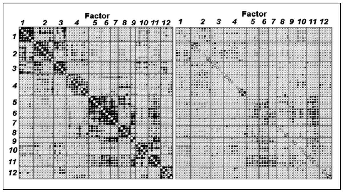
Figure 8. Bubble plots matrix of correlations between filtered monthly temperature anomalies in regions before (left panel) and after (right panel) fitting the factor model. Positive correlations are shown as black dots and negative correlations are shown as red dots. The size of each dot is proportional to the absolute value of the correlation coefficient.

The average changes with 95% confidence intervals (CI) of filtered monthly temperature anomalies per decade over 1973-2008 were estimated for each of the 12 large regions, as well as the five sub-regions with high uniqueness in the factor analysis, and are mapped in Figure 9. Eleven of the 12 large regions and all the five sub-regions showed a significant increase in temperature (p-values< 0.05). Each such region was reclassified into three levels according to the lower bound of the 95% CI of its temperature change per decade: small if between0.090°C and 0.129°C, moderate (0.130°C-0.199°C) and large (0.200°C-0.320°C) temperature increase. Three colors, yellow, orange and red, were used to indicate the three different levels in Figure 9.

Clearly, large temperature increases occurred in the north Pacific Ocean, Alaska and Eastern Siberia (large regions 4, 8 and 9). Increases in north Canada, Greenland, Iceland, Norway, Sweden and Finland (large regions 2, 3, 10 and 11) were moderate. Small increases occurred in northern Siberia and part of the north Atlantic (large regions 5, 6, 7 and 12), whereas northeast Canada and its surrounding seas (large region 1) did not experience much change (colored green in Figure 9). Four out of the five sub-regions (colored cream in Figure7) experienced a small temperature increase per decade, but the other sub-region, covering Severanya Zemlya, had a large temperature increase. Note that the two sub-regions with more than 80% missing data are colored blue in Figure 9.

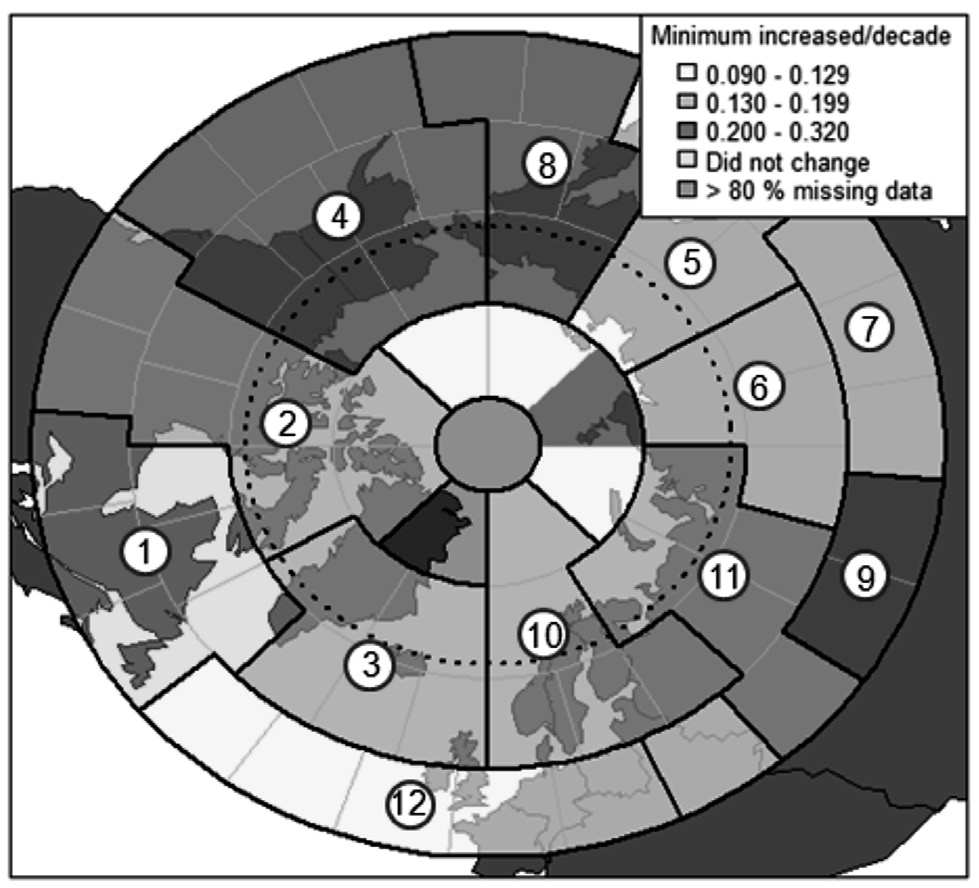
Figure 9. The minimum temperature increased per decade in regions.

DISCUSSION AND CONCLUSIONS

Twelve large regions covering 62 of the 69 sub regions studied, each with different warming patterns, were identified from our study. Some had relatively large temperature increases per decade, including the north Pacific Ocean, Alaska and Eastern Siberia. A large temperature change was also detected in Severanya Zemlya. Except for northeast Canada and its surrounding seas, almost all regions included in the study experienced some level of temperature increase.

An earlier study by Jones et al., (1999) suggested that temperature in the Northern Hemisphere rose on average by 0.37°C in 1925-1944 and 0.32°C over 1978-1997. As in Jones’s study, our study showed a temperature increase almost everywhere. Temperature increase detected in the Arctic in the present study is consistent with that from the studies of the same region over a similar period by Rigor et al., (1999) and Polyakov (2012).In addition, this study showed that rising temperature in the northern areas (land and sea) of the Atlantic, similar to that on the surface of the northern Atlantic Ocean reported recently by McNeil and Chooprateep (2013).

The results from the present research provide comprehensive information about temperature changes on the Earth’s surface close to the Arctic region (land and sea), one of the most important areas for global warming research. Any change in the Arctic may result in a substantial change in climate globally, and by the same token global change may have pronounced effects on the Arctic region. The methodological approach used in the present study can be applied to similar studies in other regions of the Earth’s surface. Furthermore, other statistical methods or techniques, such as linear spline model, T-mode PCA with K-means clustering and polynomial functions, could be utilized to extend the approach used in the current study. Although the present study only considered temperature, the approach presented here can be applied to the studies of other factors, such as solar radiation, wind, and rainfall in future studies.

ACKNOWLEDGEMENTS

The authors are grateful to Emeritus Prof. Don McNeil, Department of Statistics, Macquarie University, Australia for supervising our research.

REFERENCES

Anisimov, O.A.,V.A. Lobanov, and S.A. Reneva. 2007. Analysis of changes in air temperature in Russia and Empirical forecast for the first quarter of the 21^st century. Russian Meteorology and Hydrology 32: 620-626. DOI: 10.3103/S1068373907100020

Box, J.E., L. Yang, D.H. Bromwich, and L.S. Bai. 2009. Greenland Ice sheet Surface Air Temperature Variability: 1840-2007. America Meteorological Society 22: 4029-4049. DOI: 10.1175/2009JCLI2816.1

Chatfield, C. 1996. The Analysis of Time Series, Chapman & Hall, Melbourne. Hughes, G.L., S.S. Rao, and T.S. Rao. 2006. Statistical analysis and time-series models for minimum/maximum temperatures in the Antarctic Peninsula. The royal society 463:241-259. Doi:10.1098/rspa.2006.1766.

Houghton, J.T., Y. Ding, D.J. Griggs, M. Noguer, P.J. van der Linden, and D. Xiaosu. 2001. Climate change 2001: The Scientific Basic. Cambridge University Press, 944 pp.

Johannessen, O.M., L. Bengtsson, M.W. Miles, S.I. Kuzmina, V.A. Semenov, G.V. Alekseev, A.P. Nagurnyi, V.F. Zakharov, L.P. Bobylev, L.H. Pettersson, K. Hasselmann, and H.P. Cattle. 2004. Arctic climate change: observe and modeled temperature and sea-ice variability. Tellus 56A:328-341. DOI: 10.1111/j.1600-0870.2004.00060.x

Johnson, D.E. 1998. Applied Multivariate Methods for Data Analysts. Duxbury. Jones, P.D., M. New, D.E. Parker, S. Martin, and I.G. Rijor. 1999. Surface air temperature and its changes over the past 150 years. Reviews of Geophysics 37: 173-199. DOI: 10.1029/1999RG900002

Krupnik, I., and D. Jolly. 2002. The Earth is Faster Now. Arctic Research Consortium, Fairbanks, AK.

Lean, J.L., and D.H. Rind. 2009. How will Earth’s surface temperature change in future decades?. Geophysical research letters 36: L15708, Doi:10.1029/2009Glo03892. DOI: 10.1029/2009GL038932

McNeil, N., and C. Chooprateep.2013. Modeling sea surface temperatures of the North Atlantic Ocean. Theoretical and Applied Climatology. Doi:10.1007/s00704-013-0930-0.

National Academies Report. 2008. Understanding and Responding to Climate Change. Highlights of National Academies Report.

Overpick, J., K. Hughen, D. Hardy, R. Bradley, R. Case, M. Douglas, B. Finney, K. Gajewski, G. Jacoby, A. Jennings, S. Lamoureux, A. Lasca, G. MacDonale, J. Moore, M. Retelle, S. Smith, A. Wolfe, and G. Zielinski. 1997. Arctic environmental change of the last four centuries. Science 278:1251-1256. DOI: 10.1126/science.278.5341.1251

Polyakov, V.I., R.V. Brkryaev, G.V. U.S. Bhatt, R.L. Colony, M.A. Johnson, A.P. Maskshtas, and D. Walash. 2002. Variability and Trends of Air Temperature and Pressure in the Maritime Arctic, 1875-2000. American Metrological Society 16:2067-2076.

R Development Core Team. R: A language and environment for statistical computing. Vienna, Austria: R Foundation for Statistical Computing, 2009.Available at URL: http://www.R-project.org. [Accessed “1 November 2009”].

Rigor, I.G., R.L. Colony, and S. Martin. 1999. Variation in Surface Air Temperature Observations in the Arctic, 1979-97. Climate 13: 896-914. doi: 10.1175/1520-0442(2000)013<0896:VISATO>2.0.CO;2

Semenov, V.A. 2007. Structure of Temperature Variability in the High Latitudes of the Northern Hemisphere. Atmospheric and Oceanic physics 43: 744-753. DOI: 10.1134/S0001433807060023

Venables, W.N., and B.D. Ripley. 2002. Modern Applied Statistics with S. Springer.