ABSTRACT

This paper studied the monthly seasonally-adjusted surface temperature patterns in Southeast Asia from 1973 to 2008. The study area comprised 40 regions of 10° by 10° grid-boxes in latitudes 25°S to 25°N and longitudes 75°E to 160°E. The data were fitted with a second-order auto-regressive process to reduce auto-correlations at lags 1 and 2 months. Factor analysis was used to account for spatial correlation between grid-boxes, giving six contiguous layer regions that extended beyond the original study area to form larger regions. Exploration extended from latitudes 35°S to 25°N and longitudes 65°E to 160°E. Multivariate linear regression models were then fitted to data within these larger regions. Temperatures were found to have increased in all regions, with the increases ranging from 0.091 to 0.240°C per decade.

Keywords: Southeast Asia, Climate change, Time series analysis, Spatial correlation, Auto-correlations, Factor analysis, Multivariate linear regression model

INTRODUCTION

Climate change research is of considerable current interest. Questions on its general patterns, the mechanisms involved, reliable predictions and the effects of our current and future choices, remain at least partly unanswered.

For statistical predictions, the starting point is an analysis of the historic patterns, with reduction of their dimensionality. The available historic data of surface temperatures are of a high dimension, because both location and time coordinates play a role. Once dimensionality has been reduced, parsimonious model fitting may become possible and facilitate predictions. Natural ways to reduce the data include averaging over locations and averaging over time. Both approaches have been used, as seen from this review of prior research highlights.

Various methodologies have been used to study climate change, including mechanism-based computer simulation models or statistical techniques, as well as their combinations. For example, using annual averages, Jones et al. (1999) studied the surface air temperatures in both the southern and northern hemispheres. They presented global fields of surface temperature change over the two 20-year periods of greatest warming during the twentieth century, 1925-44 and 1978-97. Over these periods, global temperatures rose by 0.37°C and 0.32°C, respectively. Hansen et al. (2006) also studied trends in annual mean temperatures, finding that the average (annually and globally) surface temperature has increased approximately 0.2°C per decade in the 30-year interval 1975-2005. In Australia, Collins et al. (2000) examined trends in annual counts of extreme temperature events, showing that the frequency of warm events has generally increased over the period 1957-96, while the number of cool extremes has decreased. Taniguchi et al. (2007) evaluated subsurface temperatures in four Asian cities in order to estimate the effects of surface warming due to urbanization and global warming, as well as the developmental stage of each city, over the periods 1991, 1992, 2003 and 2006. Mean surface warming in each city ranged from 1.8 to 2.8°C: Bangkok (1.8°C), Osaka (2.2°C), Seoul (2.5°C) and Tokyo (2.8°C).

Numerous studies have assessed both temperature trends and spatial correlation over land surfaces. For example, Kiraly et al. (2006) investigated correlation properties of daily temperature anomalies over land. Several thousand temperature records from the Global Daily Climatology Network were analysed by means of detrended fluctuation analysis (DFA). Short-range correlations were also evaluated by DFA and by first order autoregressive models. The strength of short- and long-range temporal correlations seemed to be coupled for large geographic areas. The spatial patterns were quite complex and had no simple dependence on, for example, elevation or distance from oceans.

Various statistical analyses have been used to model patterns of temperature change. For instance, Anisimov et al. (2007) investigated changes in air temperature in Russia. The spatial homogeneity of air temperature anomalies within each region were assessed through coefficients of correlation between the regionally averaged temperature time series and series at each station of this region, over the periods 1900-49 and 1950-2004. The minimum coefficient of multiple correlation was found to be 0.8. Hughes et al. (2006) studied the variations in the minimum/maximum temperatures of the Antarctic region using a multiple regression model with non-Gaussian correlated errors and linear autoregressive moving average (ARMA) models with innovations. The innovations had an extreme value distribution. This analysis showed an increase in the minimum monthly temperature of approximately 6.7°C over 53 years (1951-2003), without significant increase in the maximum temperatures. Griffiths et al. (2005) investigated extreme temperature changes in the Asia-Pacific region over the period 1961-2003, covering latitudes 46°N - 47°S and longitudes 80°E - 120°W. This study focused on the relationship between mean and extreme temperature in the Asia-Pacific region. The daily temperature time series were used to compute annual averages and annual standard deviations for maximum and minimum temperature. Trends and relationships were calculated using linear regression and Pearson correlation analysis.

The aim of this study is to investigate the trends and patterns in temperatures of a large specific region of Southeast Asia from 1973 to 2008. The selected region includes both land and sea, and temperature profiles of adjacent locations are correlated. Time series analyses use a simple linear model. To observe and make use of the correlations between adjoining areas, we aggregate data from adjoining regions and fit models to data in larger regions. Thus, there is a fine location mesh at which pre-processed measurement data is available and a coarser mesh in which we generate temperature values by within subregion averaging. Factor analysis and a multivariate linear regression model are used in the spatial analysis. The linear model is also used to predict temperature changes over the next decade.

MATERIALS AND METHODS

Monthly temperatures in Southeast Asia for the 36-year period were obtained from the Climate Research Unit (CRU, 2009) and described in detail by Brohan et al. (2006). CRU provides monthly temperature averages for 5° by 5° latitude-longitude grid-boxes on the earth’s surface, based on data collected from weather stations, ships and, more recently, satellites. The data incorporates 40 regions of 10° by 10° grid-boxes which were designed like ice-blocks in an igloo. These areas are located in latitude 25°S to 25°N and longitude 75°E to 160°E, and compose of all or part of 11 Southeast Asian countries, including: northern Australia, southern India, Bangladesh, Nepal, Bhutan, southern China, the Indian Ocean and the western Pacific Ocean, as shown in Figure 1. 

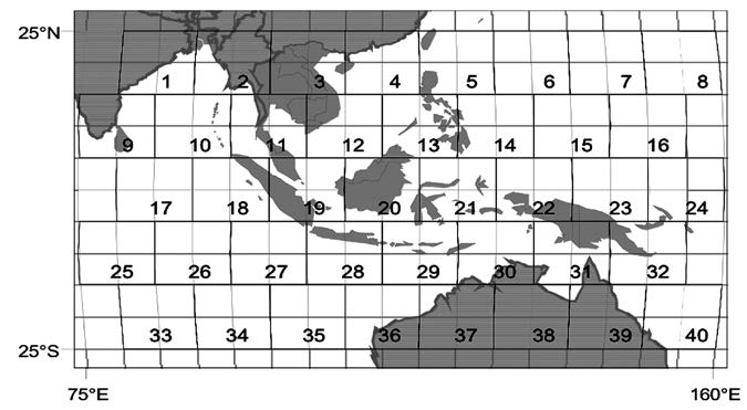
Figure 1. The study region.

Statistical methods

The data consist of 432 monthly temperatures, which were seasonally adjusted. For each grid-box, seasonal variation was removed by subtracting the monthly average and then adding back the overall mean temperature. Using a simple linear model to fit these seasonally-adjusted temperatures (Figure 3), the model takes the form:

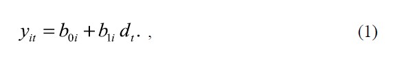
where y_it denotes the seasonally-adjusted temperature in grid-box i for month t and d_t denotes the time elapsed in decades since 1973, centered at the middle of the period, that is, d_t = (t –n/2)/120 for a period of n months, b_0i is the average temperature in grid-box i over the period and b_1i is the estimated rate of increase in temperature per decade.

The auto-correlation coefficients measure the correlations between successive observations at different lags. The average monthly temperatures were filtered to remove auto-correlations at lags 1 and 2 months using the filter (Chatfield, 1996):

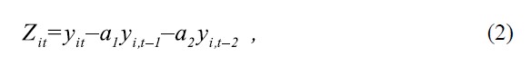
where coefficients a₁ and a₂ are obtained by fitting auto-regressions with two parameters to the data for each grid-box.

Factor analysis (Mardia et al., 1980) allocates variables into groups by maximizing correlations between variables within the same group and minimizing correlations between variables in different groups. This method was applied to identify correlations between the filtered monthly temperatures in the 40 grid-boxes into groups with different climate change patterns. Grid-boxes with uniqueness (the proportion of the variability that is not shared with the other variables) greater than 0.88 were omitted from the factor analysis. The factor model formulation with p factors takes the form:

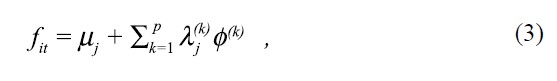
where are adjusted temperatures in month i and grid-box j, μ_j is the mean temperature of variables in grid-box j,  are the factor loadings at grid-box j on the k^th factor and  are the common factors (Table 1). Data analysis and graphical displays were carried out using R (R Developement Core Team, 2009).

RESULTS

The simple linear regression model was fitted to aggregated seasonally-adjusted temperature centered to zero mean. The result in Figure 2 shows that the mean temperature increased by 0.159°C per decade over the 36-year-period, with correlation (r) 0.59 and 95% confidence interval 0.138 - 0.180°C.

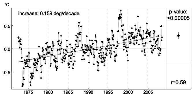
Figure 2. Mean temperature change using simple linear regression model.

Separate linear models were fitted to the seasonally adjusted temperatures for each of the 40 grid-boxes of the Southeast Asia region. Figure 3 shows that the temperatures in each grid-box have increased over the 36-year-period.

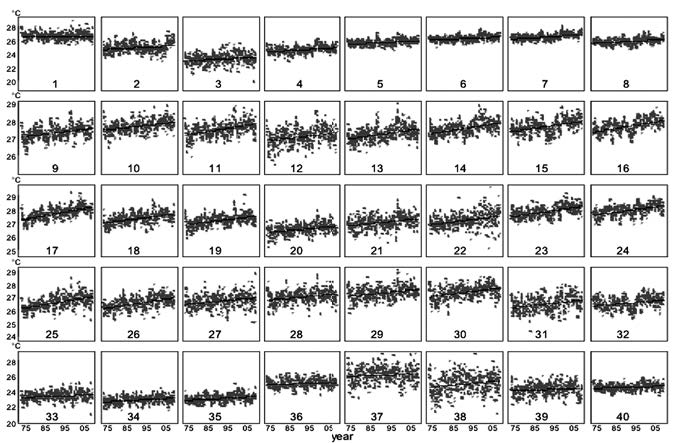
Figure 3. Temperature trends for each region, using simple linear regression
models.

In the time-series analysis, the correlations in residuals from this fitted model are assumed to be stationary.

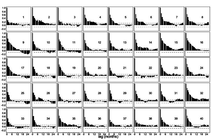
Figure 4. Auto-correlation function plots for the 40 grid-boxes.

The ACF plots in Figure 4 show that all auto-correlations are positive up to lag 26, with many being significant. To account for these significant auto-correlations, an auto-regressive process of order two was fitted to the residuals from the linear regression model.

The average values of the two parameters in the fitted 2-term auto-regressive models are a₁ = 0.494 and a₂ = 0.107; the filter has removed the auto-correlation structure as shown in Figure 5.

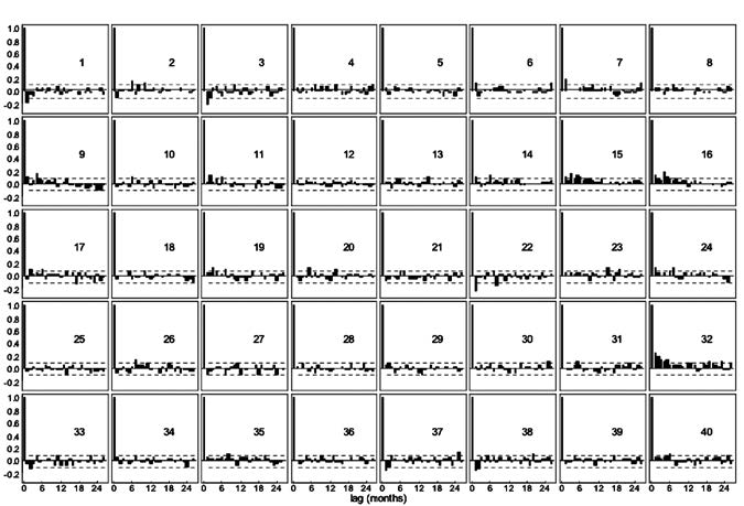
Figure 5. Auto-correlation functions for the filtered residuals.

Table 1. Results of the factor analysis.

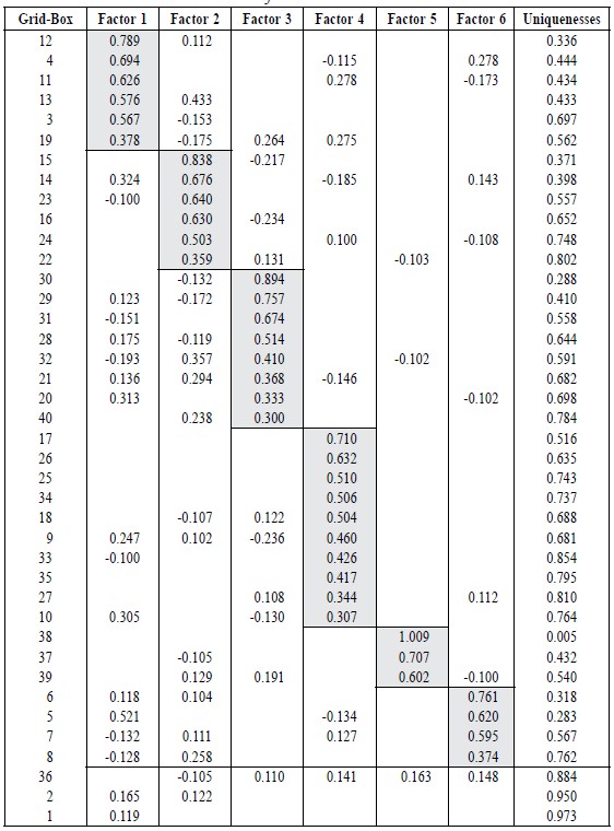
The factor analysis gave six groups of filtered temperatures in grid-boxes comprising 6, 6, 8, 10, 3 and 4 of grid-boxes, respectively. The high loadings have been highlighted with shading. There are four grid-boxes that have a mix of factors, and three grid-boxes that have high uniqueness.

Figure 6 shows high correlations of the filtered temperatures within each  factor order by six factors (left). The factor model can reduce these correlations as shown in the correlation of the residuals (right).

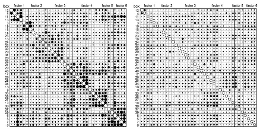
Figure 6. Bubble plots of correlations between filtered monthly temperatures in grid-boxes before (left) and after (right) fitting the factor model.

Of the 40 grid-boxes, 37 could be classified by factor analysis and combined into six regions, which are displayed in the upper part of Figure 7. Further exploration extended the area by 10° in each direction: north, south, east and west. By factor analysis, 46 from 54 of the adjoining grid-boxes were combined, as shown in the lower part of Figure 7 (after first omitting those not correlated). All the regions stay the same, except some grid-boxes.

Each factor comprised the followings regions:

• Factor 1: Southern China, Vietnam, Cambodia, Thailand, Laos, Malaysia, Singapore and Philippines.

• Factor 2: Western Pacific Ocean.

• Factor 3: Indonesia and Papua New Guinea.

• Factor 4: Southern India, Sri Lanka and the Indian Ocean.

• Factor 5: Northern Australia.

• Factor 6: Northwest Australia and the Eastern Indian Ocean

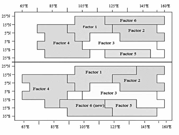
Figure 7. The adjoining grid-boxes were combined into six regions.

Multivariate linear regression models were used to fit parameters for each factor. The response variables are filtered temperatures of each grid-box in the same factor and the explanatory variable is 432 months elapsed. These models provide variance-covariance matrices of estimated temperature increases in adjoining grid-boxes of each factor. A simple linear regression model was used to analyse the average temperatures; estimated parameters are the mean estimated parameter for each relevant factor based on the average for boxes of that factor’s area.

Figure 8 shows that the temperatures increased in each factor at the 95% confidence interval for the change per decade, ranging from 0.091 to 0.240°C per decade. Figure 9 shows the 95% confidence intervals for the predicted temperature change from 2009-18 for all regions in the same graph. Factor 5 had the highest range of predicted temperatures, about 0.7°C (21.8°C to 22.5°C), while Factor 2 had the lowest range, about 0.1°C (27.8°C to 27.9°C).

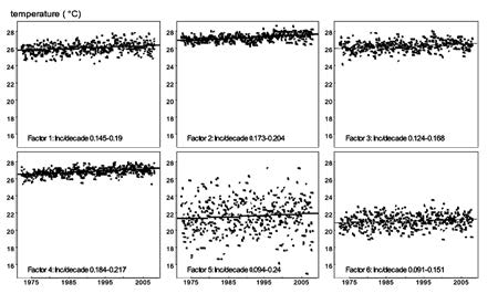
Figure 8. Temperature changes in regions defined by factors.

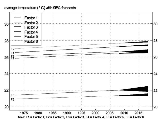
Figure 9. Temperature changes, with 95% confidence intervals, for the predicted temperature change in the next decade.

DISCUSSION

The average monthly temperatures in Southeast Asia from 1973 to 2008 were analyzed using various methods: a simple linear model, a multivariate linear regression model and factor analysis. A Linear model was fitted to the seasonallyadjusted temperatures using data collected from forty 10° by 10° grid-boxes, covering latitudes 25°S to 25°N and longitudes 75°E to 160°E. The temperatures were filtered by removing the auto-correlation using an AR(2) process. Because of correlations between residuals in adjoining grid-boxes (spatial correlation), factor analysis was used to classify filtered monthly temperatures in grid-boxes into six regions. Multivariate linear regression model was used to fit parameters for each factor. In the extended area covering latitudes 35°S to 25°N and longitudes 65°E to 160°E factor analysis could be classified by six similar regions, except some grid-boxes. A fit of trend of each region by simple linear model, showed that temperatures have increased gradually on average during 1973-2008. Simple linear regression models were also used to predict temperature in each region in the next decade (2009-18). Region 5 had the highest range of predicted temperatures with 0.7°C.

Future studies could investigate temperature changes over longer periods using linear spline models. Moreover, the study could be extended from Southeast Asia to other areas of the world.

ACKNOWLEDGEMENTS

We are grateful to Emeritus Prof. Don McNeil for supervising our research.

REFERENCES

Anisimov, O.A., V.A. Lobanov, and S.A. Reneva. 2007. Analysis of changes in air temperature in Russia and Empirical forecast for the first quarter of the 21^st century. Russian Meteorology and Hydrology. 32(10): 620-626.

Brohan, P., J. J. Kennedy, I. Harris, S. F. B. Tett, and P. D. Jones. 2006. Uncertainty estimate in regional and global observed temperature changes: A new data set from 1850. Geophysical research.111: D12106, doi:10.1029.

Chatfield, C. 1996. The Analysis of Time Series, Chapman & Hall, Melbourne. Collins, D.A., P.M. Della-Marta, N. Plummer, and B.C. Trewin. 2000. Trends in annual frequencies of extreme temperature events in Australia. Australian Meteorology Magazine. 49: 277-292.

CRU. 2009. Climatic Research Unit, School of Environmental Sciences, University of East Anglia, Norwich, UK. Retrieved April 1, 2010, from http://www.cru.uea.ac.uk/cru/data/temperature.

Griffiths, G.M., L.E. Chambers, M.R. Haylock, M.J. Manton, N. Nicholls, H.J. Baek, Y. Choi, P.M. Della-Marta, A. Gosai, N. Iga, R. Lata, V. Laurent, L. Maitrepierre, H. Nakamigawa, N. Ouprasitwong, D. Solofa, L. Tahani, D.T. Thuy, L. Tibig, B.Trewin, K. Vediapan, and P. Zhai. 2005. Change in mean temperature as a predictor of extreme temperature change in the Asia-Pacific region, J. Climatol. 25: 1301-1330.

Hansen, J., M. Sato, R. Ruedy, K. Lo, D.W. Lea, and M. Medina-Elizade. 2006. Global temperature change. PNAS. 103. 14288-14293. 

Hughes, G.L., S.S. Rao, and T.S. Rao. 2006. Statistical analysis and time-series models for minimum/maximum temperatures in the Antarctic Peninsula, The royal society, doi:10.1098/rspa.2006.1766.

Jones, P.D. M. New, D.E. Parker, S. Martin, and I.G. Rijor. 1999. Surface air temperature and its changes over the past 150 years. Reviews of Geophy-sics. 37: 173-199

Kiraly, A., I. Bartos, and I.M. Janosi. 2006. Correlation properties of daily temperature anomalies over land, J Tellus. 58A: 593-600.

Mardia, K.V., J.T. Kent, and J.M. Bibby. 1980. Multivariate Analysis, Academic Press Inc. (London) Ltd.

R Development Core Team. 2009. R: A language and environment for statistical computing. Vienna, Austria: R Foundation for Statistical Computing, Available at URL: http://www.R-project.org. [Accessed “1 November 2009”]

Taniguchi M., T. Uemura, and K. Jago-on. 2007. Combined effects of urbanization and global warming on subsurface temperature in four Asian cities. Vadose Zone Journal. 6: 591-596.