ABSTRACT

Land Surface Temperature (LST) data around Kathmandu Valley of Nepal from 2000 to 2015 were analyzed to determine the temperature patterns. The cubic spline function was used to find the seasonal patterns, which were similar for all sub-regions, with a single summer peak and a winter trough. The data were then seasonally adjusted to remove seasonal effects and filtered with the first-order autocorrelation. The second-degree polynomial regression model identified fifteen different patterns; 65.4% of the area had an ‘accelerating’ pattern and 34.6% had a ‘non-accelerating’ pattern. The logistic regression confirmed that the patterns were significantly associated with altitude (P = 0.006). This study identified a varying pattern of temperature by location and time and the methods can be generalized to larger areas. 

Keywords: Land Surface Temperature, Cubic spline function, Polynomial regression model, Temperature patterns

INTRODUCTION

Temperature change, a crucial environmental problem, can hit low-income countries hard, with their reliance on natural resources. Warming of the land surface is particularly problematic, as it directly affects the surrounding ecosystem. The land surface temperature is both related to and can affect a range of natural and human activities, including agriculture (Schlenker and Roberts, 2009; Smith et al., 2009), health (Dhimal et al., 2015; Xu et al., 2015), the environment (Jones et al., 1999; Johannssen et al., 2004), and energy (Paniagua-Tineo et al., 2011; Jaglom et al., 2014); it affects every sphere of human life.

Global surface air temperatures were predicted to show a continuous rise from 2009 to 2019 (Lean and Rind, 2009). The average surface temperature of the earth has increased 0.65-1.06°C from 1880-2012, with land surfaces increasing the most to the combined effect of natural and human forces (Intergovernmental Panel on Climate Change [IPCC], 2013). Despite its wide scope and importance, the mechanisms, trends, and patterns of temperature change are not fully understood. The literature has identified temperature change through annual seasonal patterns (Portmann et al., 2009) and trends (Hughes et al., 2006; Devkota, 2014), but the analysis of annual temperature patterns that explain the characteristics of the change is limited. However, reliable and complete data is challenging to obtain, especially in low-income countries, where field data inventory systems are limited. In this situation, remote sensing or satellite data provide the best alternative; one of the common satellite-based data sets is the Land Surface Temperature (LST) from Moderate Resolution Imaging Spectroradiometer (MODIS) (Wan et al., 2004).

Temperature data have been analyzed in several ways, including simulation models (Johannessen et al., 2004), remote sensing algorithms (Li et al., 2013), and various statistical techniques (Hughes et al., 2006; Dong et al., 2014; Me-ead and McNeil, 2016). Wanishsakpong and McNeil (2016) used a polynomial regression model to investigate trends and patterns of temperatures in Australia. More recently, Wongsai et al. (2017) used cubic spline to investigate annual seasonal patterns and decadal trends of LST data.

Nepal is vulnerable to climate change effects because of its ecologically, biologically, and geographically diverse regions (Anup and Ghimire, 2015). The maximum temperature increased 0.03°C on average per year in summer and 0.05°C in winter from 1978 to 2008 (Joshi et al., 2011). The growing urban region around Kathmandu Valley is suffering from unmanaged human encroachment and excessive pollution (United Nations [UN]-Habitat, 2015); this is affecting temperatures. Although, temperature variations and trends have been studied in Nepal (Sano et al., 2005; Shrestha and Aryal, 2011; Devkota, 2014), no study has analyzed annual temperature patterns around the valley itself. In fact, global or regional climate change analyses usually average away local variability and, thus, cannot represent local variations of temperature (IPCC, 2013). Therefore, this study aimed to identify comprehensive patterns of temperature  change and analyze their association with altitude locally around the Kathmandu Valley over a 15-year period (2000-2015). It is assumed that altitude has some relationship with the temperature change pattern in general (Shrestha and Aryal, 2011; Lancaster, 2012; Stroppiana et al., 2014).

MATERIALS AND METHODS

The study area extends around the central coordinate of 27.595°N and 85.394°E, covering an area of 3,969 km² around the Kathmandu Valley of Nepal (Figure 1). It is a hilly region with temperate climate and has three distinct annual seasons – winter, summer, and rainy fall. Kathmandu is the fastest growing and most populated city in Nepal, with a population density of 2,731/km²; the peripheral area of valley has a density of 275/km² (NPHC 2011, 2012). The south of Nepal contains a belt of hot plains, with the altitude gradually increasing moving north; the temperature declines with increasing elevation (United Nations Environment Program [UNEP], 2001).

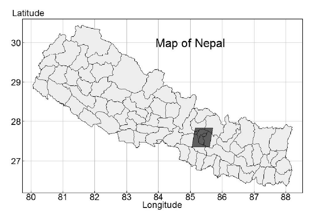
Figure 1. Map of Nepal showing the study area (shaded box).

Land Surface Temperature data

The Land Surface Temperature (LST) data for nine regions, representing the total study area, were retrieved from the MODIS website (Oak Ridge National Laboratory Distributed Active Archive Center [ORNL DAAC], 2015). MODIS is a sensor aboard the Terra and Aqua satellites of the National Aeronautics and Space Administration (NASA). It monitors environmental changes globally due to fire, vegetation, temperature, earthquakes, drought, and floods (NASA, 2015). LST data has dynamic range, high radiometric resolution, and is accurately calibrated (Wan et al., 2004). The spatial resolution of the LST data used for each region was a 1×1 km² grid. The covered area extended 10 km from the center in all four directions (east, west, north, and south). As a result, the study area covered 21×21 km², with 441 grids of 1 km² each.

The LST data were retrieved one-by-one for each of the nine regions for a period from May 2000 to June 2015 in eight-day intervals, or approximately 46 observations per year and maximally 690 observations over the 15-year period. Due to technical problems with sensors, 9.68% of the observations were missing across the nine regions over the period, so the actual total count of observations for each grid cell was typically below the maximum. Figure 2 shows the nine regions; each region was divided further into nine sub-regions of approximately 7×7 km² each, or 49 grids; this ensured more detail to detect changing patterns in a smaller area. The LST data for each sub-region were taken as an average of 49 grids for every observation to reduce spatial correlation and represent temperature for each sub-region. The average LST were analyzed for each of the 81 sub-regions. The central region shows an example of the sub-regions (Figure 2), which were named North-East (NE), North (N), North-West (NW), West (W), Central (C), East (E), South-West (SW), South (S), and South-East (SE) based on their locations.

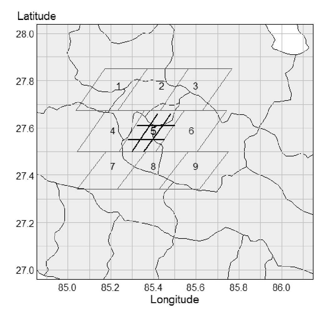
Figure 2. Study area of nine regions and the sub-regional division in center.

Altitude data

The altitude data for 81 sub-regions were obtained from Google Earth. First, nine different location points or their coordinates were calculated systematically, as a three-bythree matrix in each sub-region. The altitudes of all these points were retrieved from Google Earth Images. These nine altitudes from each sub-region were averaged to get a single altitude to represent a particular sub-region. The altitudes ranged from 435 m to 2,245 m, which were grouped into two categories – below or above 1,500 m – and hence the altitude variable became binary.

Statistical methods 

A cubic spline function was fitted with a selected number of knots to find the seasonal temperature patterns. The function took the form:

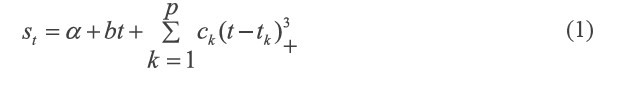
Where, α, b, and c_k are the parameters in the model. t denotes time in Julian days, that is, specified day of year. t₁ < t₂ < ... < t_p are specified knots and (t-t_k)+ is t-t_k for t > t_k and 0 otherwise.

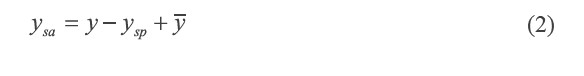
The temperature data were seasonally adjusted by subtracting the spline fitted values (y_sp) from the temperature (y) and then adding back the mean of the temperature  of each sub-region. The formula took the form:

The dependencies among the seasonally adjusted temperature data were reduced by removing the auto-correlations at the lag 1 term (equivalent to an eight-day period). The autocorrelation at the lag 1 term (a₁) is shown in Figure 5. The data were then filtered (Me-ead and McNeil, 2016; Wanishsakpong and McNeil, 2016). The filtered temperature data were finally fitted with a polynomial regression model of second degree (quadratic model). The model took the form:

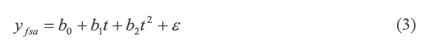
where b₀ is the constant and b₁ and b₂ are the coefficients. The time of observation was represented by t and ε is the error term. The estimated temperature increase or decrease was calculated based on the first derivative of the quadratic function.

All the temperature patterns obtained from equation 3 were then categorized into a binary form (accelerating or nonaccelerating pattern). The association between the temperature patterns and altitude of the study area was identified using a logistic regression model that took the form:

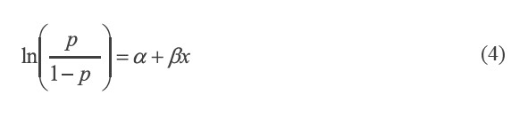
where p denotes the expected probabilities of the accelerating temperature pattern, α is the intercept, x is the determinant variable that is altitude, and β is the regression coefficient.  Eighty-one observations were used to construct the model.

R Statistical Programming (R Core Team, 2015) was used to analyze the data and generate the graphics.

RESULTS

The annual seasonal patterns of LST were quite similar and the cubic spine showed little variation across the nine regions. The central region is used as an example in Figure 3 to explain the seasonal temperature pattern of every sub-region. Nine panels represent the sub-regions and eight positive (+) signs at the bottom of each panel show the knot positions. Each vertical gray line represents an observation day and the black dots are the temperature plotted consecutively for 15 years. In each panel, a smooth spline curve (gray line) is derived from the cubic spline model with r2 ranging from 0.50 to 0.81. The temperature began to rise immediately after winter in February and the peak was seen during summer in March, April, and May (days 80 to 140). By the end of May, it gradually declined and reached the trough in winter during December, January, and February (days 350 to 40).

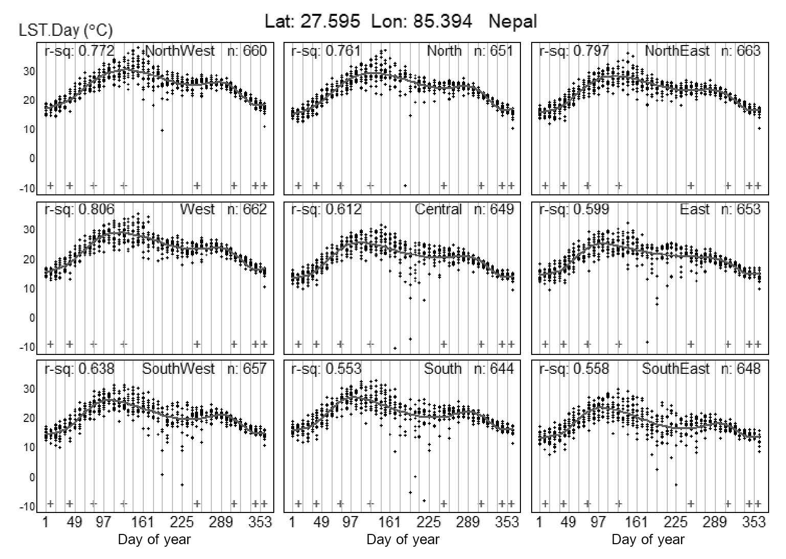
Figure 3. Cubic spline function showing seasonal patterns of temperature changes in the nine sub-regions of the central region during days 1 to 365.

Figure 4 illustrates the 81 seasonal temperature patterns. Each panel represents the nine sub-regions of the respective region represented by different types of lines. Each line type represents a particular location of the sub-region. The seasonal patterns were similar across locations, except slight variations in temperature levels in regions two, eight, and nine.

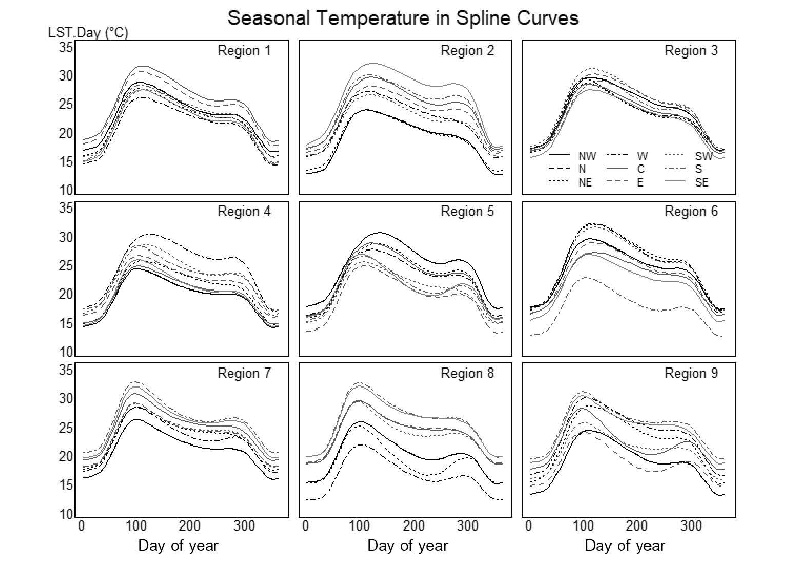
Figure 4. Seasonal temperature patterns of the 81 sub-regions within the respective nine regions.
Note: Lines represent particular locations within the sub-region – black solid for NW, black dashed for N, black dotted for NE, black dot-dash for W, gray solid for C, gray dashed for E, gray dotted for SW, gray dot-dash for S, and light gray for SE sub-regions.

Seasonally-adjusted, filtered temperature data for every sub-region were subjected to the quadratic model; Figure 5 shows an example using the central region. It illustrates the quadratic curves of nine sub-regions in nine different panels. The tenth panel, on the bottom right side, shows all those curves in nine different types of lines, one for each sub-region. During the 15-year period, the study area showed a net rise of temperature ranging from 0.009 to 0.430 °C and a fall from -1.047 to -0.010 °C, along with the auto-correlations (a1) of the data below 0.35.

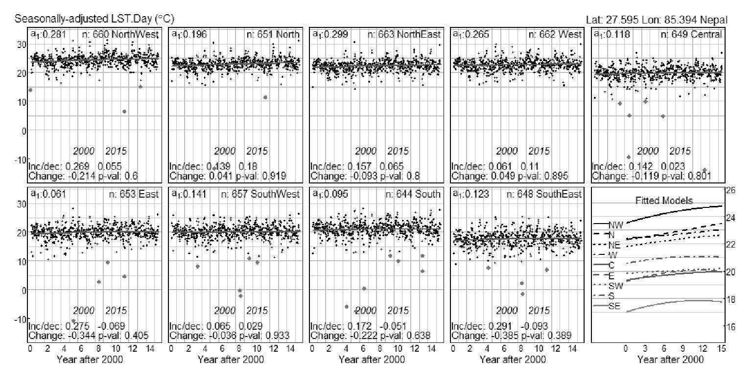
Figure 5. Temperature patterns of the nine sub-regions of the central region.
Note: The y-axis shows seasonally adjusted temperature in degree Celsius (°C); the x-axis represents the years from 2000 to 2015; n is the number of observations in each sub-region; a₁ is the autocorrelation of sub-region level data; and inc/dec shows the increase or decrease of temperature per decade, with its difference between 2000 and 2015 providing the total linear change of the temperature over the 15-year period. The P-values of the quadratic model in each sub-region are also shown.

The quadratic curves of the temperatures in 81 sub-regions, plotted together in a map of the study area (Figure 6), showed 15 different patterns; these were categorized into two groups based on their shape. The first one was an ‘accelerating’ pattern that covered 65.43% of the area; the other one was ‘non-accelerating’ that covered 34.57% of the area. The accelerating pattern included all the patterns that were in rising tendency ; the non-accelerating pattern included the remainder, including thorough declining , recently declining , or no changes . All of them were supposed to impart no risk effects to the environment.

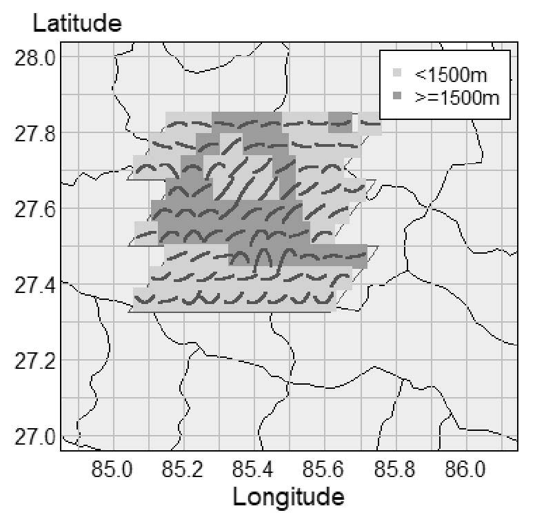
Figure 6. Temperature patterns of 81 sub-regions with altitude levels.

Along with the temperature patterns, Figure 6 also shows the altitudes (shaded area) in the region. Here, 60.49% of sub-regions had altitudes lower than 1,500 m and the rest had higher altitudes. The core center, that is the Kathmandu Valley, was surrounded by high altitudes, while the remainder had lower altitude. The logistic model applied to these variables showed that the temperature patterns were negatively associated (regression coefficient = -1.36, P-value = 0.006) with the altitude of the site. That is, the accelerating temperature slopes were found to associate mostly with the lower altitudes and vice versa (Figure 6). Figure 7 illustrates the 95% confidence interval plot after the logistic model; it shows that the accelerating temperature pattern was more likely to associate with lower altitude areas. 

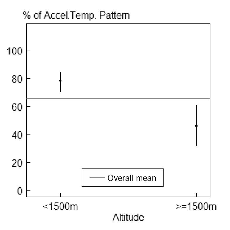
Figure 7. Confidence intervals plot showing the association between temperature pattern and altitude.

DISCUSSION

This study applied a combination of cubic spline function and polynomial regression model to analyze temperature patterns using MODIS LST time series data for the Kathmandu Valley of Nepal. Cloud cover and rainy seasons caused uncertain and missing values in the LST time series. It has been suggested that the cubic spline function can be used to detect the seasonality in MODIS LST time series data; the cubic spline function helped extract annual seasonality, even with missing values in the time series (Wongsai et al., 2017). Since MODIS provides LST time series data for each grid (1×1 km²), the cubic spline can be applied to each LST time series (of every grid). In this study, the LST data for each sub-region were aggregated and analyzed. Moreover, the sub-region level results can be obtained for any extent of area coverage (each region can be bigger than 21x21 km²) and any length of time.

The seasonal temperature patterns showed almost similar peaks (in summer) and troughs (in winter) in all sub-regions, suggesting that they did not vary in those locations. Portmann et al. (2009) observed a contrasting result in the distribution of temperature patterns in the USA; they showed that annual maximum and minimum temperature trends varied significantly at different sites, but over larger areas; this variation was associated with rainfall. The temperature can be higher or lower depending on topography (Fu and Rich, 2002) or land cover (Yue et al., 2007), as well. The seasonal patterns in our study detected variations of temperature levels for panels 2 and 8 only; these might have been due to climatic factors like topography, rainfall, altitude, or land cover.

Stroppiana et al. (2014) showed that the trend of LST could be explained by a simple linear regression model. However, a linear model might not be the most appropriate method to estimate trends for shorter periods. A polynomial pattern of temperature was identified in Australia from 1970 to 2012 (Wanishsakpong and McNeil, 2016); they used a 6^th degree polynomial regression model because the data covered more than 40 years. Within 40 years, 15-year periodic temperature patterns were well explained; hence, our study, with its shorter time frame, was able to use a polynomial with lower degree (2^nd). Hence, the annual temperature patterns illustrated in 15 groups are more interesting in this study. The patterns suggested that the local variation of temperature change in the study area might be due to the effect of different natural (vegetation, altitude, and topography) and human factors (land use and urban activities). The southern and central sub-regions had an accelerating pattern. Both of these regions were at lower altitudes with dense populations. In contrast, the northern and western area, both at higher altitudes, had a ‘non-accelerating’ pattern. In the literature, analyzing temperature data on the regional or global scale is common to determine trends (Hughes et al., 2006; Devkota, 2014) or patterns (Zhou et al., 2009; Wanishasakpong and McNeil, 2016), but the results do not illustrate local patterns within the much larger study areas. Macro-level spatial analysis, while valuable, overlooks localized changes. This study improves the understanding of temperature patterns in a much smaller area – the Kathmandu Valley – and provides a basis for urban planning and environmental management at the local level.

Several studies have found an association between temperature and elevation (Fu and Rich, 2002; Pouteau et al., 2011; Stroppiana et al., 2014). The correlation is greater in winter and lower in summer; but not consistent throughout the year or over the study periods. In our study, the logistic model aimed to explain the higher probability of an accelerating temperature pattern at lower altitude. Our results were consistent with Stroppiana et al. (2014) that temperature change and patterns are negatively associated with altitude. Lancaster (2012) found the same relationship in Malawi with altitudes from 900 m to 2,400 m). In contrast, Shrestha and Aryal (2011) showed that the rising temperature change was progressive towards the higher altitudes in the Himalayan glacial region of Nepal, an area mostly higher than 4,000 m; this extreme altitude might be the cause of the contrast with our results. In China, Dong et al. (2014) found that the temperature was decreasing below an altitude of 200 m, increasing from 200-2,000 m, and weakly positive above 2,000 m. Although altitude and temperature change has a strong statistical relationship, these studies have shown that it can be either positive or negative, depending on altitude, topography, or land use pattern.

Since Nepal is highly dependent on natural resources and agriculture, slight changes in temperature and rainfall pattern make it more vulnerable to climate change (Anup, 2014). Finding the causal factors of variation in the pattern of LST change needs a very detailed micro-level analysis that is beyond the scope of this paper.

CONCLUSION 

This study applied a cubic spline function and polynomial regression model, accounting for seasonal adjustment and autocorrelation effects in data, to find temperature patterns on a small or local, as opposed to regional or global, scale. Although the seasonal patterns (intra annual) were comparatively consistent with respect to the nearby locations, the annual temperature patterns varied considerably. The 15 different patterns of temperature change identified in this study were more effective in explaining the actual path (pattern) of temperature change than linear trends.

ACKNOWLEDGEMENTS 

This work was supported by the Higher Education Research Promotion and the Thailand’s Education Hub for Southern Region of ASEAN Countries Project Office of the Higher Education Commission (grant number, TEH-AC 018/2015). We acknowledge the Department of Mathematics and Computer Science of Prince of Songkla University for providing facilities for this study. We are grateful to Professor Don McNeil for his immense guidance during the study.

REFERENCES

Anup, K.C. 2014. Climate change communication in Nepal. In: Filho, W.L., Manolas, E., Azul, A.M., Azeiteiro, U.M, and McGhie, H. (ed.) Handbook of climate change communication. Springer, Switzerland. p. 21-36.

Anup, K.C., and Ghimire, A. 2015. High-altitude plants in era of climate change: A case of Nepal Himalayas. Chapter 6. In: Ozturk, M., Hakeem, K., Faridah-Hanum, I., Efe, R. (eds.). Climate Change Impacts on High-Altitude Ecosystems. Springer, Cham. p. 176-187. https://doi.org/10.1007/978-3-319-12859-7_6

 
Devkota, R.P. 2014. Climate change: trends and people’s perception in Nepal. Journal of Environmental Protection. 5: 255-265. https://doi.org/10.4236/jep.2014.54029

Dhimal, M., Ahrens, B., and Kuch, U. 2015. Climate change and spatiotemporal distributions of vector-borne diseases in Nepal- a systematic synthesis of literature. PLOS ONE. 10(6): 1/31-6/31. https://doi.org/10.1371/journal.pone.0129869

Dong, D., Huang, G., Qu, X., Tao, W., and Fan, G. 2014. Temperature trend-altitude relationship in China during 1983-2012. Theoretical and Applied Climatology. 122(1): 285-294. https://doi.org/10.1007/s00704-014-1286-9

Fu, P., and Rich, P.M. 2002. A geometric solar radiation model with applications in agriculture and forestry. Computers and Electronics in Agriculture. 37: 25-35.

Hughes, G.L., Rao, S.S., and Rao, T.S. 2006. Statistical analysis and time-series models for minimum/ maximum temperatures in the Antarctic Peninsula. The Royal Society. 463: 241-259. https://doi.org/10/1098/rspa.2006.1766

IPCC. 2013. Climate Change 2013: The physical science basis. Contribution of working group I to the fifth assessment report of the Intergovernmental Panel on Climate Change. Cambridge United Kingdom and New York, USA. Retrieved from http://www.climatechange2013.org/images/report/WG1AR5_ALL_FINAL.pdf

Jaglom, W.S., McFarland, J.R., Colley, M.F., Mack, C.B., Venkatesh, B., Miller, R.L., Haydel, J., Schultz, P.A., Perkins, B., Casola, J.H., et al. 2014. Assessment of projected temperature impacts from climate change on the U.S. electric power sector using the Integrated Planning Model. Energy Policy. 73: 524–539. https://doi.org/ 10.1016/j.enpol.2014.04.032

Johannessen, O.M., Bengtsson, L., Miles, M.W., Kuzmina, S.I., Semenov, V.A., Alekseev, G.V., Naguarnyi, A.P., Zakharov, V.F., Bobylev, L.P., Pettersson, L.H., et al. 2004. Arctic climate change: observe and modeled temperature and sea-ice variability. Tellus. 56: 328-341. https://doi.org/10.1111/j.1600-0870.2004.00060.x

Jones, P.D., New M., Parker, D.E., Martin, S., and Rijor, I.G. 1999. Surface air temperature and its changes over the past 150 years. Reviews of Geophysics. 37: 173-199. https://doi.org/10.1029/1999RG900002

Joshi, N.P., Maharjan, K.L., and Piya, L. 2011. Effect of climate variables on yield of major food-crops in Nepal -A time-series analysis. MPRA. Paper No. 35379, posted 15 December 2011. Retrieved from https://mpra.ub.uni-muenchen.de/35379/

Lancaster, I.N. 2012. Relationships between altitutude and temperature in Malawai. South African Geographical Journal. 62(1): 89-97. https://doi.org/10.1080/03736245.1980.10559624 

Lean, J.L., and Rind, D.H. 2009. How will Earth’s surface temperature change in future decades? Geophysical Research Letter. 36: L5708. https://doi.org/10.1029/2009GLo38932

Li, Z.L., Tang, B.H., Wu, H., Ren, H., Yan, G., Wan, Z., Trigo, I.F., and SobrinoLi, J.A. 2013. Satellite-derived land surface temperature: Current status and perspectives. Remote Sensing of Environment. 131: 14–37.

Me-ead, C., and McNeil, N. 2016. Graphical display and statistical modeling of temperature changes in tropical and subtropical zones. Songklanakarin Journal of Science and Technology. 36 (6): 715-721.

NASA. 2015. Global Climate Change: Vital Signs of the Planet. Retrieved from http://climate.nasa.gov/effects

NPHC. 2011, 2012. National Survey Report. 1: 3-40. Central Bureau of Statistics. Government of Nepal, Kathmandu.

ORNL DAAC. 2015. MODIS subset of NASA Earth Data. Retrieved from: http://daacmodis.ornl.gov/cgi-bin/MODIS/GLBVIZ_1_Glb/modis_subset _order _global_col5.pl.

Paniagua-Tineo, A., Salcedo-Sanz, S., Casanova-Mateo, C., Ortiz-Garcia, E.G., Cony, M.A., and Hernandez-Martin, E. 2011. Prediction of daily maximum temperature using a support vector regression algorithm. Renewable Energy. 36: 3054-3060. https://doi.org/10.1016/j.renene.2011.03.030

Portmann, R.W., Solomon, S., and Hegerl, G.C. 2009. Spatial and seasonal patterns in climate change, temperatures, and precipitation across the United States. Proceedings of National Academy of Sciences of United States of America (PNAS). 106(18): 7324–7329. https://doi.org/10.1073/pnas.0808533106

Pouteau, R., Rambal, S., Ratte, J.P., Goge, F., Joffre, R., and Winkel, T. 2011. Downscaling MODIS-derived maps using GIS and boosted regression trees: The case of frost occurrence over the arid Andean highlands of Bolivia. Remote Sensing of Environment. 115: 117–129. http://dx.doi.org/10.1016/j.rse.2010.08.011

R Core Team. 2015. R: A language and environment for statistical computing. R Foundation for Statistical Computing, Vienna, Austria. Retrieved from http://www.R-project.org/

Sano, M., Furuta, F., Kobayashi, O., and Sweda, T. 2005. Temperature variations since the mid-18th century for western Nepal, as reconstructed from tree-ring width and density of Abies spectabilis. Dendrochronologia. 23: 83–92. https://doi.org/10.1016/j.dendro.2005.08.003

Schlenker, W., and Roberts, M.J. 2009. Nonlinear temperature effects indicate severe damages to U.S. crop yields under climate change. Proceedings of National Academy of Sciences of United States of America (PNAS). 106(37): 15594–15598. https://doi.org/10.1073/pnas.0906865106

Shrestha, A.B., and Aryal, R. 2011. Climate change in Nepal and its impact on Himalayan glaciers Regional Environmental Change. Regional Environmental Change. 11(suppl.1): 65–77. https://doi.org/10.1007/s10113-010-0174-9

Smith, J.B., Schneider, S.H., Oppenheimer, M., Yohe, G.W., Hare, W., Mastrandrea, M.D., Patwardhan, A., Burton, I., Corfee-Morlot, J., Magadza, C.H.D., et al. 2009. Assessing dangerous climate change through an update of the Intergovernmental Panel on Climate Change (IPCC) “reasons for concern”. Proceedings of National Academy of Sciences of United States of America (PNAS). 106(11): 4133–4137.

Stroppiana, D., Antoninetti, M., and Brivio P.A. 2014. Seasonality of MODIS LST over Southern Italy and correlation with land cover, topography and solar radiation. European Journal of Remote Sensing. 47(1): 133-152. https://doi.org/10.5721/EuJRS20144709

UNEP. 2001. Nepal: state of the environment. p. 12-13. Retrieved from http://www.rrcap.ait.asia/Publications/nepal%20soe.pdf

UN-Habitat. 2015. Cities and climate change initiative, abridged report: Kathmandu Valley, Nepal. United Nations Human Settlements Program, Nairobi, Kenya.

Wan, Z., Wang, P., and Li, X. 2004. Using MODIS Land Surface Temperature and Normalized. Difference Vegetation Index products for monitoring drought in the southern Great Plains, USA. International Journal of Remote Sensing. 25(1): 61-72. https://doi.org/10.1080/0143116031000115328

Wanishsakpong, W., and McNeil, N. 2016. Modelling of daily maximum temperatures over australia from 1970 to 2012. Meteorological Applications. 23: 115-122. https://doi.org/10.1002/met.1536

Wongsai, N., Wongsai, S., and Huete, A.R. 2017. Annual seasonality extraction using the cubic spline function and decadal trend in temporal daytime Modis lst data. Remote Sensing. 9: 1254. https://doi.org/10.3390/rs9121254

Xu, Z., Jiang, Y., and Zhou, G. 2015. Response and adaptation of photosynthesis, respiration, and antioxidant systems to elevated CO₂ with environmental stress in plants. Frontiers in Plant Science. 6: 701. https://doi.org/103389/fpls.2015.00701

Yue, W., Xu, J., Tan, W., and Xu, L. 2007. The relationship between land surface temperature and NDVI with remote sensing: application to Shanghai Landsat 7 ETM+ data. International Journal of Remote Sensing. 28(15): 3205–3226. https://doi.org/10.1080/01431160500306906

Zhou, L., Dickinson, R.E., Dirmeyer, P., Dai, A., and Min, S.K. 2009. Spatiotemporal patterns of changes in maximum and minimum temperatures in multi-model simulations. Geophysical Research Letters. 36: L02702. https://doi.org/10.1029/2008GL036141