ABSTRACT 

This study investigated the effect of different sub-division schemes and two rainfall data types – gauge and radar – on the accuracy of runoff forecasting using a semi-distributed hydrological URBS model in a large river basin with a limited network of rainfall gauges. The entire catchments at three runoff stations in the Upper Ping River Basin, Thailand, were employed initially as a single lumped unit, and each catchment was thereafter divided into four increasingly complex subdivision schemes. Model performance was compared using areal gauge rainfall data (from the sparse rain gauge network) and estimated, high-resolution, radar rainfall data across all catchment schemes over three periods; June-October 2003, May-September 2004, and May-July 2005. The results indicated that the accuracy of runoff estimates increased with increasing catchment subdivision complexity when using the high-resolution radar rainfall, but did not improve with the rain gauge data.

Keywords: Catchment subdivision, Radar rainfall, Rain gauge rainfall, Semi-distributed model

INTRODUCTION 

Hydrological modelling is a non-structural tool for predicting water runoff in a catchment basin. The models are of three types: lumped, semi-distributed, and distributed (Cunderlik, 2003; Jajarmizadeh et al., 2012). The lumped model is the simplest; it assumes that precipitation and model parameters are uniform over the basin. The larger the basin and more variable its characteristics, the less accurate this model becomes (Koren et al., 1999). The semidistributed model allows for partial spatial variations in precipitation, streamflow routing, and catchment by sub-dividing the catchment area; this improves predictive performance (Boyle et al. 2001). The distributed model allows the modeler to specify the spatial resolution over which to fully vary the model parameters; this provides the most accurate runoff estimates, but is highly complex, requiring significant data parameterization (Arnold et al., 1998). Researchers develop models with higher degrees of structural complexity in the expectation of improving prediction accuracy (Perrin et al., 2001; Mayr et al., 2013). However, more complicated models normally require more input data, and are difficult to apply, especially for catchments with insufficient or no hydrologic data. In addition, the more complex the model, the more difficult it is to assess its parameters, leading to large parameter uncertainty (Butts et al., 2004). As such, the semi-distributed model offers a reasonable compromise between simplicity and complexity for estimating water runoff in areas with limited measuring networks.

Factors associated with rainfall and catchment characteristics significantly affect the accuracy of runoff estimation (Wilson, 1979; Hamlin, 1983). Semi-distributed models with complex catchment subdivision schemes can help account for the spatial variation of rainfall and catchment characteristics, such as topography, land use, or soil properties (Ajami et al., 2004). However, several studies found that high-resolution sub-catchments do not necessarily improve model performance for a variety of reasons, including the theories and concepts of the selected models being compared, the sensitivity and uncertainty of model parameters, catchment and climate characteristics, and data quality (Han et al., 2013; Zhang et al., 2013).

This study focuses on the effect of rainfall data quality on the accuracy of runoff modelling in a country, Thailand, with a limited capacity/network to measure continuous ground rainfall – a major constraint to effective modeling. Rain gauge measurements from this sparse network cannot spatially represent rainfall distribution over the basin. As such, this study investigated whether adding more structural complexity (by subdividing the catchment into finer scale) to only coarse resolution of rainfall gauge data could lead to a better model and simulation results. We also investigated whether combining higher resolution rainfall data from radar, as opposed to ground gauges, with finer resolution of sub-catchments would improve model results. Our research then demonstrated the relative benefits offered by applying gauge and radar rainfall data to different catchment subdivision scales to simulate the runoff hydrograph in the Upper Ping River Basin, Thailand.

MATERIALS AND METHODS

Semi-distributed model

This study used the Unified River Basin Simulator (URBS), a semi-distributed, nonlinear, rainfall-runoff-routing model that can account for the spatial and temporal variation of rainfall. Carroll (2007) developed the URBS model based on research by Laurenson and Mein (1990). Both the Australian Bureau of Meteorology and the Chiangjiang (Yangtze) Water Resources Commission in China have used the model to forecast floods (Malone, 2003; Jordan et al., 2004; Pengel et al., 2007). Mapiam and Sriwongsitanon (2009) used the URBS model for flood estimation on the gauged catchments in the Upper Ping River Basin; they later formulated a relationship for using the model on the ungauged catchments of the basin. Subsequently, Mapiam et al. (2014) applied the URBS model with three types of radar and rain gauge rainfall inputs with different temporal and spatial resolution to investigate the best model for flow simulation in the Upper Ping River Basin. They found that radar rainfall data was more accurate than rain gauge data for estimating hourly runoff of the overall flow hydrographs.

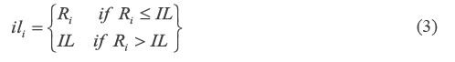
Using the URBS mode, this study first divided the catchment (study area described below) into sub-catchments. The excess rainfall estimation for each sub-catchment was later calculated using an initial loss – proportional runoff model (IL-PR) for pervious areas and a spatial infiltration model for impervious areas. The accumulated rainfall depth at the beginning period of simulation (R_i) was deducted by an initial loss (mm) until the R_i exceeded the maximum initial loss (IL, mm). The proportional loss using proportional runoff coefficient (pr, dimensionless) was incorporated. The pervious excess rainfall depth at time t (R_t ^per) was given by:

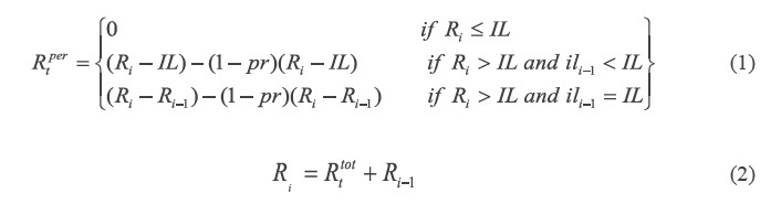
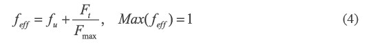
where R_{t ^tot} is the rainfall depth during a time interval (Δt) – 1 hour in this study. The accumulated initial loss at time t (il_i) was described as below:

The effective fraction of the area that is impervious (f_eff ) was given by Equation 4:

where f_u is existing fraction of the impervious area (this study assumed f_u = 0), F_t is the cumulative infiltration into the pervious area starting from the beginning of a simulation period, F_max is the maximum infiltration capacity of the sub-catchment (IF parameter). Excess rainfall (R_t) at time t on the corresponding sub-catchment was calculated using Equation 5:

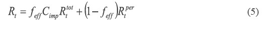
where C_imp is the impervious runoff coefficient (the default is 1) and  R_{t ^per} is calculated using the IL-PR model.

After determining excess rainfall for each sub-catchment, we conventionally applied the catchment routing and channel models to estimate runoff at the outlet using Equations 6 and 7, respectively:

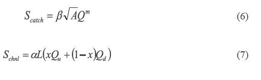
where for Equation 6,  S_catch is the catchment storage (m³s^-1 h) of each sub-catchment, β is the catchment lag parameter (h/km) for each sub-catchment, A is an area of sub-catchment (km²), m is the dimensionless catchment non-linearity parameter, and Q is the outflow of catchment storage (m³/s) of the corresponding sub-catchment. For Equation 7, S_catch is the channel storage (m³s^-1 h) for each sub-catchment, α is the channel lag parameter (h/km) for each sub-catchment, L is the length of a reach (km) considered in channel routing, Q_u is the inflow at the upstream end of a reach (including sub-catchment inflow, Q, calculated using Equation 6), Q_d is the outflow at the downstream end of a channel reach (m³s^-1) of the corresponding sub-catchment, and x is the Muskingum translation parameter.

From Equations 1 to 7, seven parameters are required to run the model: channel lag (α), catchment nonlinearity (m), Muskingum translation (x), catchment lag (β), initial loss (IL), proportional amount of runoff (PR), and maximum infiltration rate (IF). Parameters α , m, x, and β are related to runoff routing and IL, PR, and IF are related to rainfall loss modelling. Since the values of m and x do not normally vary significantly from 0.8 and 0.3,
respectively (Carroll, 2007; Jordan et al., 2004), we used these values in our model. The other five parameters (α, β, IL, PR, and IF) were determined during calibration and verification.

Study areas and data collection 

The study area was three point locations – runoff stations P.21, P.24A, and P.71 – in the Upper Ping River Basin, Thailand. The basin landform is undulating terrain. The catchment areas of these three stations are approximately 515, 460, and 1,771 km2, respectively (Figure 1). Rainfall data was collected from 35 daily rain gauges in the study area, owned and operated by the Royal Irrigation Department and the Thai Meteorological Department. The study used radar reflectivity data from the Omkoi Radar, owned and operated by the Department of Royal Rainmaking and Agricultural Aviation. The continuous runoff data was collected from that recorded at stations P.21, P.24A, and P.71. Locations of rain gauge runoff stations and the radar radius are shown in Figure 1.

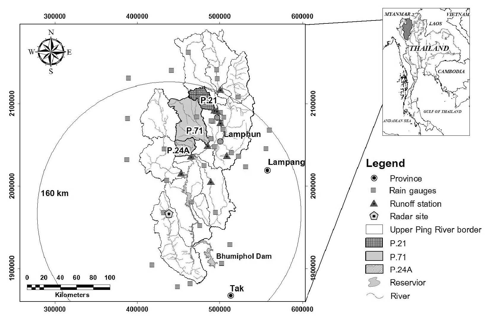
Figure 1. The locations of the gauge catchment areas (P.21, P.24A, and P.71), radar, rain gauges, and runoff stations.

Catchment subdivision schemes

To investigate the effect of the degree of structural complexity on runoff modelling, the gauge catchments over the three runoff stations (P.21, P.24A, and P.71) were each divided into sub-catchments to enhance model complexity. A series of catchment subdivision levels were configured by considering topography and catchment characteristics. Five subdivision schemes were then constructed by delineating each sub-catchment into an equivalent size as the percentage of the whole area of each gauge catchment as follows: 100% (scheme-100%), 50% (scheme-50%), 25% (scheme-25%), 12% (scheme-12%), and 7% (scheme-7%) of the whole area. Locations of the centroid of each sub-catchment at each scenario were specified and the distance from the centroid to the outlet of the corresponding sub-catchment, or centroid length, was then calculated for constructing river network schematization. Total rainfall depth and calibrated model parameters were assumed to be uniform over each sub-catchment. Two alternative rainfall measures – gauge and radar rainfall data – were assessed at the subcatchment level (described in the next section) and used in the URBS model to convert to excess rainfall using Equations 1-5. The estimated excess rainfall over a sub-catchment was routed through the catchment storage, located at the centroid of that sub-catchment, to the channel using the catchment routing technique, as shown in Equation 6; afterward, the outflow from the catchment storage, which is the inflow of channel storage (Q_u) was routed along a reach (the centroid length) to the next downstream sub-catchment, using the Muskingum method (Equation 7). The number of sub-catchments (NSC), the sub-catchment area (SCA), and the centroid length (CL) are the three sub-catchment variables needed to construct the catchment network at each catchment subdivision scheme in the URBS model. The subcatchment variables corresponding to each catchment subdivision scheme at each runoff station are presented in Table 1 and Figure 2.

Table 1. Sub-catchment variables of the URBS model for each catchment subdivision scheme.

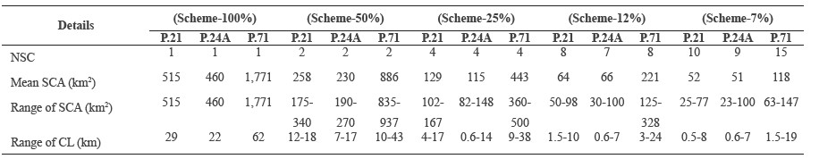
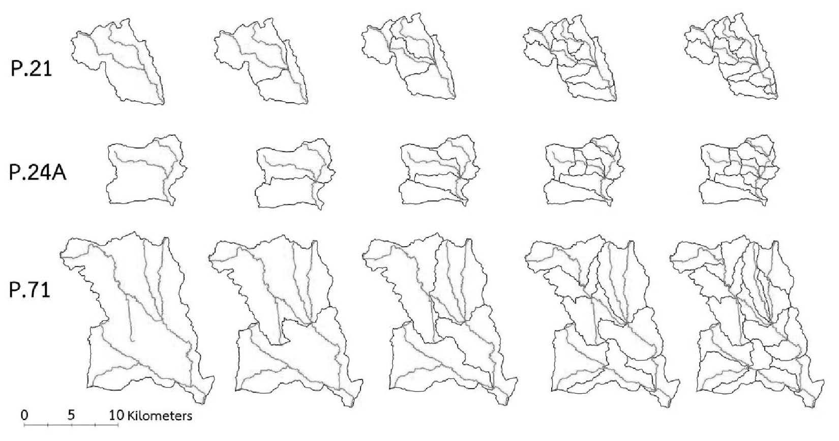
Figure 2. Catchment subdivision schemes for P.21, P.24A, and P.71 catchments.

Assessment of rainfall inputs

This study used two different measures of rainfall input distributed over each subcatchment area – gauge rainfall and radar rainfall. Data from these parameters from June-October 2003 were used to calibrate the model. Data from May-September 2004 and May-July 2005 were used to verify the model.

Gauge rainfall. Daily gauge rainfall data located within 160 km from the Omkoi radar was collected for analysis. The data were controlled for quality by considering rainfall data from adjacent gauges and ensuring consistency in the ensuing double mass curves. If unusual rainfall data were found, these were excluded from the analysis. Rain gauge data of acceptable quality was then spatially averaged using the Inverse Distance Weighting (IDW) technique for each sub-catchment. IDW is a simple interpolation approach that has been widely used in many applications (Dirks et al., 1998; Chinchorkar et al. 2012). Under conditions of insufficient data density, IDW performs better than other statistical interpolation methods like multiple linear regression, optimal interpolation, or Kriging (Eischeid et al., 2000). Catchment studies with a limited rain gauge network select IDW to assess areal rainfall.

Radar rainfall. Weather radar has been used as an alternative tool for providing high-resolution spatial and temporal rainfall estimates, especially in areas with insufficient rainfall stations, like Thailand, in order to enhance flood prediction accuracy. Mapiam and Sriwongsitanon (2008) first developed a climatological Z-R relationship (Z=74R^1.6) based on daily data for converting instantaneous reflectivity data into rainfall rate in the Upper Ping River Basin. However, Mapiam et al. (2009) found that using the daily (24-hour) Z-R relationship to estimate hourly radar rainfall can lead to significant errors when estimating extreme rainfall. To reduce this error, the scale-transformed hourly Z-R relationship (Z=88R^1.6) proposed by Mapiam et al. (2009) has been recommended for estimating hourly radar rainfall; it improves overall runoff estimates (Mapiam et al., 2014). Before applying the reflectivity data with the Z-R relationship, radar reflectivity measurement errors need to be eliminated. Since the Omkoi radar used in this study is an S-band Doppler radar, beam attenuation error was assumed to be insignificant (Hitschfeld and Bordan, 1954; Delrieu et al., 2000). To avoid the bright band effect, we only used radar reflectivity data within 160 km of the radar.

The effect of ground clutter and beam blocking was eliminated by using a topography map of known ground clutter locations and discarding radar measurement in these areas. The effect of noise and hail in the measured radar reflectivity was addressed by assuming reflectivity values less than 15 dBZ to represent a reflectivity of 0 mm⁶ m^-3, and those greater than 53 dBZ to equal 53 dBZ, respectively. After eliminating these errors, the radar reflectivity data was converted into radar rainfall by applying the relationship Z=88R^1.6 at all pixels located in the three gauged catchments. The radar rainfall for each sub-catchment with a 1 km2 spatial resolution was estimated by averaging radar rainfall of all pixels located within a considered sub-catchment using a simple arithmetic averaging method.

Parameterization of the URBS model

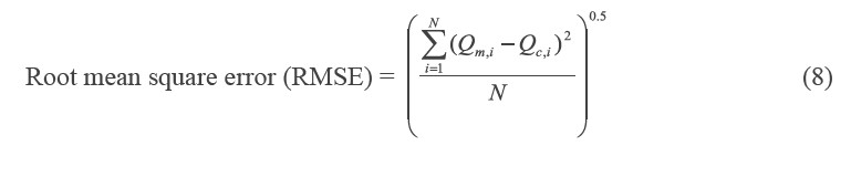
Model calibration and verification followed conventional procedures to ascertain the five control parameters (α, β, IL, PR, and IF) of the URBS model corresponding to each rainfall data set (guage and radar) and catchment sub-division scheme. The calculated rainfall during June-October 2003 was used to calibrate the model; data from May-September 2004 and May-July 2005 was used to verify the model. Unfortunately, the URBS model cannot be calibrated automatically. To reach the optimal set of model parameters for each scenario, we thus applied a simple optimization technique called a grid-base parameter search developed by Mapiam et al. (2014). Overall root mean square error (RMSE) between the calculated and measured discharges for each simulation case was used as the objective function, as shown in the following equation:

To evaluate the performance of each rainfall type and catchment structural complexity based on the calibrated parameter application, the hourly calculated and observed hydrograph at each gauge catchment were compared using the determination coefficient (R²) and efficiency index (EI) or Nash-Sutcliffe criterion (Nash and Sutcliffe, 1970), as presented in Equations 9-10:

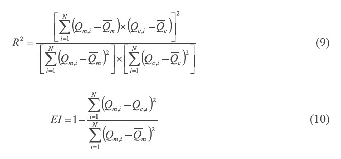
where, Q_m,i is the observed discharge at time i,  is the average value of the observed discharge, Q_c,i is the calculated discharge at time i,  is the average value of the calculated discharge, and N is the number of data points. The best fit between calculated and observed discharges using these parameters occurs when the correlation coefficient (r) approaches 1, the efficiency index (EI) approaches 100%, and the overall root mean square error (RMSE) approaches zero.

RESULTS 

Model calibration and verification 

The results of model calibration based on the algorithm mentioned above explicitly showed that the calibrated model parameters changed with the source of rainfall data (gauge or radar) and the catchment sub-division schemes, as presented in Table 3. The set of the model parameters for each simulation case determined from model calibration was then validated using data from May-September 2004 and May-July 2005 to determine whether the calibrated model parameters could be applied to other rainfall events. The results of three statistical measures comparing the simulated and observed discharges for each gauge catchment and each rainfall data type during calibration and validation periods are summarized in Table 4. Examples of time series plots comparing observed and calculated flow hydrographs during the calibration and verification periods at runoff station P.24A are presented in Figures 3-4, respectively.

Table 3. Set of the calibrated model parameters for different model structure and rainfall measurement types.

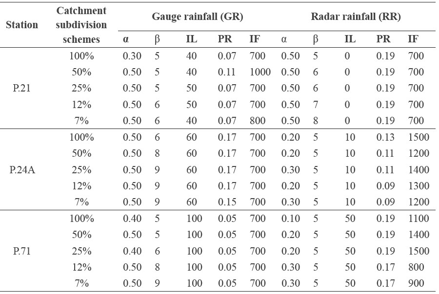
Table 4 indicates that the accuracy of the calculated flow hydrographs changed with simulation periods, spatial and temporal distribution of rainfall measurement types, and catchment structural complexity. Applying the calibrated model parameters without adjusting the values reduced the accuracy of the results in the verification period compared to the calibration period, as shown by the mostly increasing R2 and EI values. Figures 3 and 4 show the differences in the runoff hydrograph patterns derived from the two types (gauge and radar) of rainfall measurements. The radar rainfall better estimated runoff than the gauge rainfall for data between August 17 – September 16, 2003, while the inverse applied for data between July 3-18, 2003. The estimated runoff hydrographs for different subdivision schemes appeared similar based on the subjective evaluation; it was difficult to identify the accuracy of runoff estimates.

Table 4. Statistical measures during the calibration and verification periods for each simulation scenario.

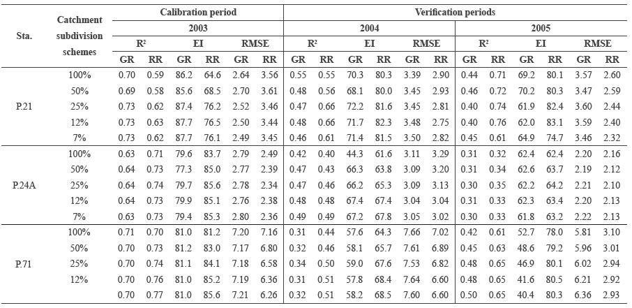
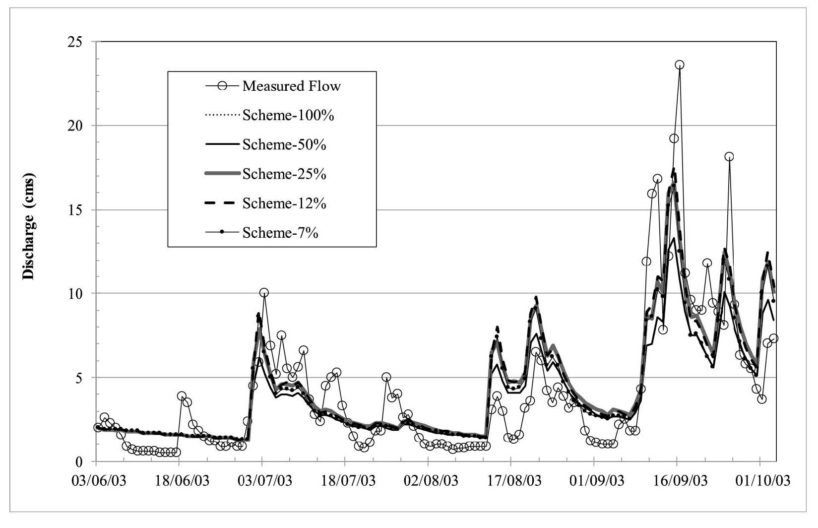
Figure 3. Calculated flow hydrographs using the gauge rainfall data at the P.24A catchment during the calibration period.

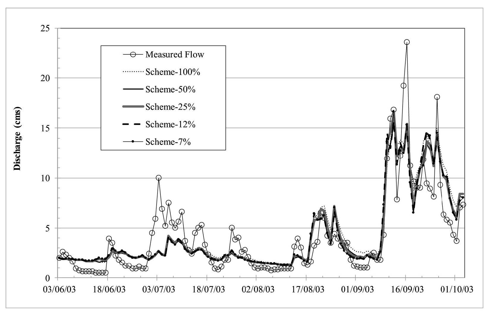
Figure 4. Calculated flow hydrographs using the radar rainfall data at the P.24A catchment during the calibration period.

Effects of catchment subdivision complexity and rainfall resolution on runoff estimates

Since this research aimed to investigate the influence of increasing model complexity (by changing the number of sub-catchments) and using alternative rainfall types (gauge and radar measurements) on the performance of runoff modelling, the simulation scenario which gave the best fit between simulated and measured hydrographs was considered most suitable. To test this, only the catchment subdivision schemes and rainfall resolution (gauge and radar rainfall) were changed, and the model parameters (α, β, IL, PR, and IF) were fixed for the analysis at each runoff station. Ten different sets of model parameters significantly changed with the subdivision scheme and rainfall input for each runoff station (Table 3). To avoid a biased outcome from the analysis, each set of model parameters was used to simulate 10 sets of flow hydrographs using the 5 subdivision schemes and 2 rainfall data types as inputs. As a result, the model was run 10 × 5 × 2 (one hundred) times for each runoff station and each data period, and the accuracy of overall flow hydrographs among all simulation cases was evaluated using RMSE, as summarized in Tables 5-7.

Table 5. Performance of runoff estimation for different simulation cases at P.21 based on average RMSE (m³/s).

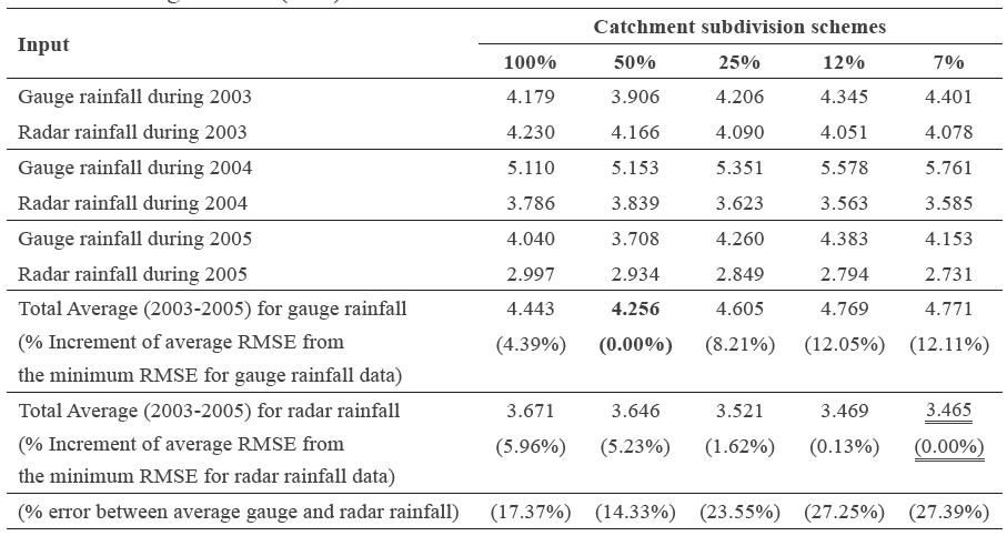
Note: The scenarios in which gauge rainfall (bold) and radar rainfall (double underline) provided the minimum average RMSE are indicated.

Table 6. Performance of runoff estimation for different simulation cases at P.24A based on average RMSE (m³/s).

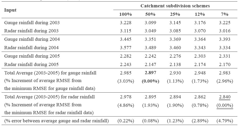
Note: The scenarios in which gauge rainfall (bold) and radar rainfall (double underline) provided the minimum average RMSE are indicated.

Table 7. Performance of runoff estimation for different simulation cases at P.71 based on average RMSE (m³/s).

Note: The scenarios in which gauge rainfall (bold) and radar rainfall (double underline) provided the minimum average RMSE are indicated.

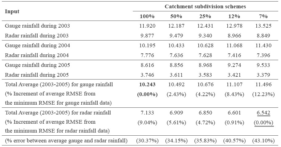
The average RMSE values among five subdivision schemes at the specific simulation period for each rainfall measurement type and runoff station were compared to assess the relative benefits of using the two types of rainfall input data (Tables 5-7). To ensure the effectiveness of model structural complexity and rainfall resolution on runoff estimates, the percentage of an increment of the average RMSE from the minimum RMSE (among five catchment network schemes) of each rainfall measurement type was considered.

For gauge rainfall, the scheme-50% provided the best average RMSE at stations P.21 and P. 24A and the scheme-100% at station P.71; the most complex scheme (scheme-7%) did not provide the minimum at any runoff station. In contrast, the radar rainfall generated the minimum average RMSE using the most complex scheme (scheme-7%) at all runoff stations. For radar rainfall, the performance of scheme-12% was almost as good in most cases.

The total average RMSE (2003-05) for each rainfall category and subdivision scheme are shown in Figure 5. This shows that runoff estimate accuracy rises with increasing subcatchment complexity when using radar rainfall data, and the inverse for gauge rainfall data.

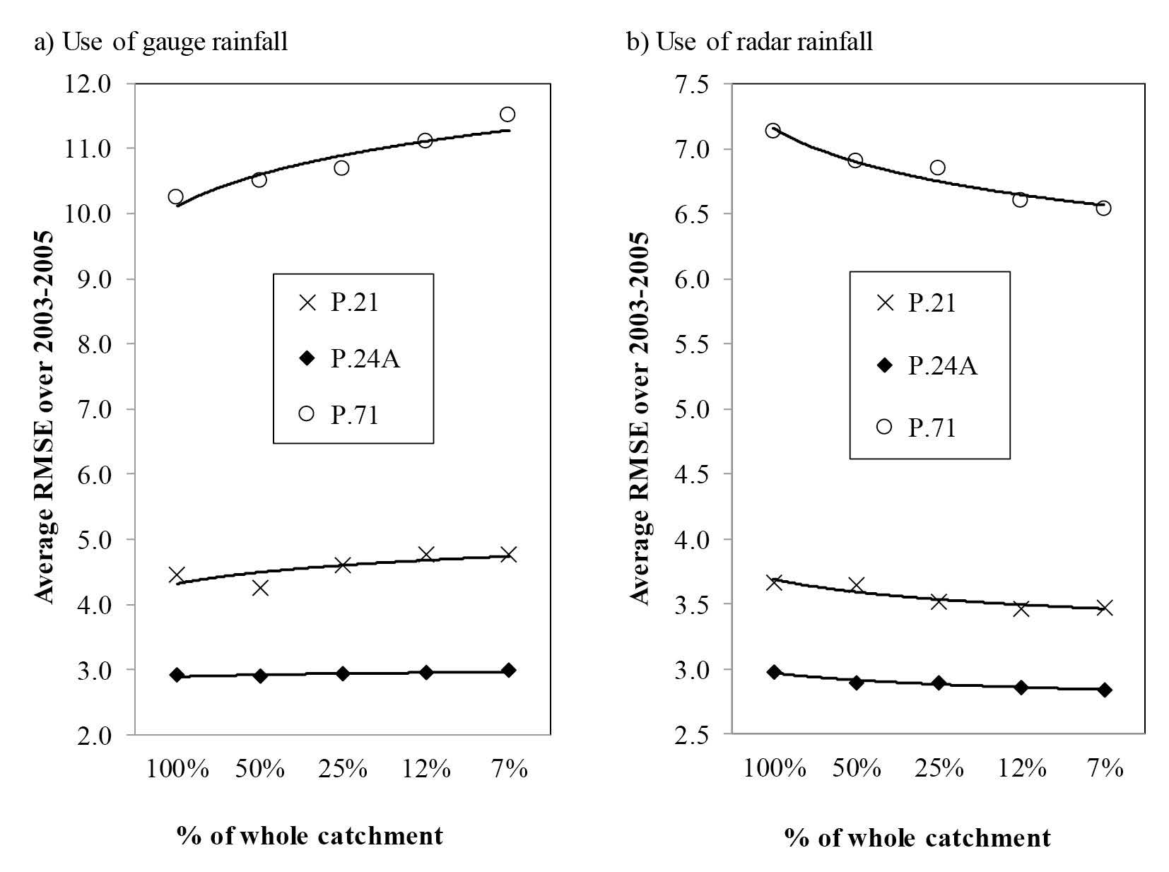
Figure 5. Comparisons of the average RMSE values of the two types of rainfall inputs for various catchment subdivision schemes.

DISCUSSION 

According to the calibration and validation results, the accuracy of streamflow estimates in the verification period were less accurate than during the calibration period. This is to be expected, because the model parameters change significantly with rainfall depths and their distribution; using the calibrated model parameters without readjustment does not represent the other perfectly. This has also been shown in other studies (Han et al., 2013; Zhang et al., 2013; Mapiam et al., 2014). We found appreciable differences in hydrograph distribution when we compared the time series plots for different resolutions of rainfall inputs (see Figures 3-4 for an example). This agreed with the assumption that the patterns of flow hydrograph are significantly influenced by the spatial and temporal distribution of rainfall (Singh, 1997; Mapiam et al., 2014).

Coupling the high resolution of the radar rainfall data with more complex sub-catchment schemes in the semi-distributed model improved the accuracy of runoff modelling. In contrast, with gauge rainfall data, increasing model structural complexity did not improve runoff estimates. This may be because the poor temporal and spatial resolution of the generated, daily, gauge rainfall data was not representative of rainfall behavior over each sub-catchment.

The highest degree of catchment subdivision complexity (scheme-7%) yielded the maximum percentage improvement (9%) in runoff estimates compared to no subdivisions (scheme-100%). Although the percentage improvement appears small, it is significant, especially for major flood events in a large river basin. As the scheme-12% provided nearly as accurate estimates as the scheme-7%, the additional structural complexity added little performance; we recommend dividing a catchment into a minimum of approximately eight sub-catchments, together with using high-resolution radar data, to improve flood forecasting in large basins with a limited ground rainfall measuring network.

REFERENCES 

Ajami N.K., Gupta, H.V., Wagner, T., and Sorooshian, S. 2004. Calibration of a semidistributed hydrologic model for streamflow estimation along a river system. Journal of Hydrology. 298(1-4): 112-135. https://doi.org/10.1016/j.jhydrol.2004.03.033

Arnold, J.G., Srinivasan, R., Muttiah, R.S., and Williams, J.R. 1998. Large area hydrologic modeling and assessment part I: Model development. JAWRA Journal of the American Water Resources Association. 34: 73-89.

Boyle, D.P., Gupta, H.V., Sorooshian, S., Koren, V., Zhang, Z., and Smith, M. 2001. Toward improved streamflow forecast: value of semidistributed modeling. Water Resources Research. 37(11): 2749–2759. https://doi.org/10.1029/2000WR000207

Butts, M.B., Payne, J.T., Kristensen, M., and Madsen, H. 2004. An evaluation of the impact of model structure on hydrological modelling uncertainty for streamflow simulation. Journal of Hydrology. 298: 242–266. https://doi.org/10.1016/j.jhydrol.2004.03.042

Carroll, D. G. 2007. URBS: a rainfall runoff routing model for flood forecasting & design version 4.30, user manual. September, 160 pp.

Chinchorkar, S.S., Patel, G.R., and Sayyad, F.G. 2012. Development of monsoon model for long range forecast rainfall explored for Anand (Gujarat-India). International Journal of Water Resources and Environmental Engineering. 4(11): 322-326. https://doi.org/10.5897/IJWREE11.097

Cunderlik, M.J. 2003. Hydrologic model selection for the CFCAS project: Assessment of water resources risk and vulnerability to changing climatic conditions, Project Report I. University of Western Ontario, Canada.

Delrieu, G., Andrieu, H., and Creutin, J.D. 2000. Quantification of path-integrated attenuation for X– and C–band weather radar systems operating in Mediterranean heavy rainfall. Journal of Applied Meteorology. 39: 840–850. https://doi.org/10.1175/1520-0450(2000)039<0840:QOPIAF>2.0.CO;2

Dirks K.N., Hay, J.E., Stow, C.D., and Harris, D. 1998. High-resolution studies of rainfall on Norfolk island part II: interpolation of rainfall data. Journal of Hydrology. 208: 187–93. https://doi.org/10.1016/S0022-1694(98)00155-3

Eischeid, J.K., Pasteris, P.A., Diaz, H.F., Plantico, M.S., and Lott, N.J. 2000. Creating a serially complete, national daily time series of temperature and precipitation for the Western United States. Journal of Applied Meteorology. 39: 1580–1591. https://doi.org/10.1175/1520-0450(2000)039<1580:CASCND>2.0.CO;2

Hamlin, M.J. 1983. The significance of rainfall in the study of hydrological processes at basin scale. Journal of Hydrology. 65: 73–94. https://doi.org/10.1016/0022-1694(83)90211-1

Han, J.C., Huang, G.H., Zhang, H., Li, Z., and Li, Y.P. 2013. Effects of watershed subdivision level on semi-distributed hydrological simulations: case study of the SLURP model applied to the Xiangxi River watershed, China. Hydrological Sciences Journal 59(1): 108–125. https://doi.org/10.1080/02626667.2013.854368

Hitschfeld, W., and Bordan, J. 1954. Errors inherent in the radar measurement of rainfall at attenuating wavelengths. Journal of Meteorology. 11: 58–67. https://doi.org/10.1175/1520-0469(1954)011<0058:EIITRM>2.0.CO;2

Jajarmizadeh, M., Harun, S., and Salarpour. M. 2012. A review on theoretical consideration and types of models in hydrology. Journal of Environmental Science and Technology. 5(5): 249-261.

Jordan, P., Seed, A., May, P., and Keenan, T. 2004. Evaluation of dual polarization radar for rainfall runoff modeling–A case study in Sydney, Australia. 6th International symposium on hydrological applications of weather radar, Melbourne, Australia.

Koren, V.I., Finnerty, B.D., Schaake, J.C., Smith, M.B., Seo, D.J., and Duan, Q.Y. 1999. Scale dependencies of hydrology models to spatial variability of precipitation. Journal of Hydrology. 217: 285–302. https://doi.org/10.1016/S0022-1694(98)00231-5

Laurenson, E.M., and Mein, R.G. 1990. RORB–version 4, runoff routing program user manual. Monash University, Department of Civil Engineering.

Malone, T., Johnston, A., Perkins, J., and Sooriyakumaran, S. 2003. Australian Bureau of Meteorology, HYMODEL – A real-time flood forecasting system. International Hydrology and Water Resources Symposium, The Institution of Engineers, Australia.

Mapiam, P.P., and Sriwongsitanon, N. 2008. Climatological Z-R relationship for radar rainfall estimation in the upper Ping river basin. ScienceAsia Journal. 34: 215–222. https://doi.org/10.2306/scienceasia1513-1874.2008.34.215

Mapiam, P.P., and Sriwongsitanon, N. 2009. Estimation of the URBS model parameters for flood estimation of ungauged catchments in the upper Ping river basin, Thailand. ScienceAsia Journal. 35: 49–56. https://doi.org/10.2306/scienceasia1513-1874.2009.35.049

Mapiam, P.P., Sriwongsitanon, N., Chumchean, S., and Sharma, A. 2009. Effect of rain–gauge temporal resolution on the specification of a Z–R relationship. Journal of Atmospheric and Oceanic Technology. 26: 1302–1314.  https://doi.org/10.1175/2009JTECHA1161.1

Mapiam, P.P., Sharma, A., and Sriwongsitanon, N., 2014. Defining the Z~R relationship using gauge rainfall with coarse temporal resolution: Implications for flood forecasting. ASCE's Journal of Hydrologic Engineering. 19(8): 04014003. https://doi.org/10.1061/(ASCE)HE.1943-5584.0000616

Mayr, E., Hagg, W., Mayer, C., and Braun, L. 2013. Calibrating a spatially distributed conceptual hydrological model using runoff, annual mass balance and winter mass balance. Journal of Hydrology. 478: 40–49. https://doi.org/10.1016/j.jhydrol.2012.11.035

Nash, J.E., and Sutcliffe, J.V. 1970. River flow forecasting through conceptual models, part 1–A discussion of principles. Journal of Hydrology. 10: 282–290. https://doi.org/10.1016/0022-1694(70)90255-6

Pengel, B., Malone, T., Tes, S., Katry, P., Pich, S., and Hartman, M. 2007. Towards a new flood forecasting system for the lower Mekong river basin. 3rd South–East Asia Water Forum, Malaysia.

Perrin, C., Michel, C., and Andréassian, V. 2001. Does a large number of parameters enhance model performance? Comparative assessment of common catchment model structures on 429 catchments. Journal of Hydrology. 242: 275–301. https://doi.org/10.1016/S0022-1694(00)00393-0

Singh, V.P. 1997. Effect of spatial and temporal variability in rainfall and watershed characteristics on stream flow hydrograph. Hydrological Processes. 11(12): 1649-1669. https://doi.org/10.1002/(SICI)1099-1085(19971015)11:12<1649::AID-HYP495>3.0.CO;2-1

Wilson, C.B., Valdes, J.B., and Rodriguez–Iturbe, I. 1979. On the influence of the spatial distribution of rainfall on storm runoff. Water Resources Research. 15: 321–328. https://doi.org/ 10.1029/WR015i002p00321

Zhang, H.L., Wang, Y.J., Wang, Y.Q., Li, D.X., and Wang, X.K. 2013. The effect of watershed scale on HEC-HMS calibrated parameters: a case study in the Clear Creek watershed in Iowa, US. Hydrology and Earth System Sciences. 17: 2735–2745. https://doi.org/10.5194/hess-17-2735-2013